Passes and Patterns: Three Downs Away: P(1D) In U Sports Football

1-Abstract

A data set of U Sports football play-by-play data was analyzed to determine the First Down Probability (P(1D)) of down & distance states. P(1D) was treated as a binomial variable, and confidence intervals were determined iteratively until convergence at the 10-10 level. For each down, fitted regression lines were added to enable discussion of overall trends with respect to distance.

Only points with a minimum N of 100 instances were considered. 1st down trended linearly, bearing only points at 5-yard intervals. 2nd and 3rd downs followed an exponential decay fit. Special attention was given to the non-zero asymptotes of these functions, and their implications towards the nature of the game. A review of & Goal data failed to provide any deeper insight.

2-Introduction

Although the study of football analytics has grown rapidly over the last 10-15 years, this research has been entirely focused on NFL and NCAA football. The discussion of P(1D) in Canadian Football is briefly covered by Taylor (2013) in a discussion of game theory and decision-making, The study of P(1D) in an American context is fairly well-trod ground, and thorough summary of this body of work has been previously published (Clement 2018a).

In this work, the dataset comes from play-by-play data accumulated from U Sports sites. The dataset was prepared and parsed to isolate the information within, a process which has been discussed in a previous work (Clement 2018b). Data was not filtered with regard to score, time remaining, or any other consideration, this being a first investigation that task was left to future researchers.

3-P(1D)

Having previously developed the dataset, a new script was developed to determine the P(1D) of different scenarios, specifically the determination of P(1D) for each combination of down & distance, while isolating & Goal scenarios. Except where otherwise specified a N=100 was used as the minimum size for each point. Admittedly an arbitrary cutoff point, there is a certain natural divide as only one point exists between N=78 and N=104, as shown in Table 1. Determination of this cutoff was made heuristically by examining the distribution of N without looking at the down & distance pairings to which they belonged to find a natural cutoff point. Since any cutoff would be arbitrary but including every data point regardless of its level of representation would be absurd this method was not considered to be significantly worse than any other.

Distance	1st Down	2nd Down	3rd Down
1	13	4107	2792
2	11	3672	759
3	9	4027	477
4	14	4594	398
5	837	5651	333
6	5	5394	247
7	8	5475	237
8	7	5029	182
9	12	4055	151
10	97932	18053	648
11	15	2537	95
12	24	1844	118
13	15	1307	70
14	29	967	78
15	1629	1494	60
16	28	708	49
17	23	611	40
18	30	473	25
19	37	381	24
20	2286	1007	52
21	18	243	16
22	8	184	16
23	9	145	6
24	7	94	9
25	236	252	13

Table 1 Distribution of Data by Down & Distance

a-code

While the notion of P(1D) is unambiguous, proper discourse demands that the methodology be publicly visible for discourse. This approach used a basic VBA script to determine the number of instances of a given scenario, how many of those were successful, and from there determine the success rate, the binomial error, and apply a weighted nearest-neighbours smoothing for use in further development.

i-Calculator

The code used to determine P(1D), shown below, exists as a subroutine within a larger program used to determine a number of other analytics. It loops over each down and distance, looking for plays that:

Match the down currently sought
Have the correct distance
Are “OD” plays
Separates by & Goal plays

The script counts the number of instances for each down & distance, and counts the number of successful iterations. It then uses those two values to populate the various tables, showing the percentage, the individual N and P values, and the exact upper and lower bounds for 95% confidence intervals, using a method discussed below.

Sub P1D_Calc()

For down = 1 To 3 'Loop through each down

For distance = 1 To 25 'Only consider distances up to 25 yds

Count = 0 'How many times this D&D has come up

success = 0 'How many times this D&D proved successful

goalcount = 0

goalsuccess = 0

For row = 2 To rowcount

If data(row, DOWN_COL) = down Then 'Check for correct D&D

If data(row, DIST_COL) = distance Then

If data(row, ODK_COL) = "OD" Then

If data(row, DIST_COL) <> data(row, FPOS_COL) Then 'Split &Goal plays

Count = Count + 1

If data(row, P1D_INPUT_COL) Then

success = success + 1

End If

Else

goalcount = goalcount + 1

If data(row, P1D_INPUT_COL) Then

goalsuccess = goalsuccess + 1

End If

Next row

P1D(distance + 1, down + 1) = success / Count 'Output the success rate

P1D(distance + 1, down + 6) = Count

P1D(distance + 1, down + 11) = success

P1D(distance + 1, down + 21) = success / Count - BinomLow(success, Count, 0.025)

P1D(distance + 1, down + 26) = BinomHigh(success, Count, 0.025) - success / Count

If goalcount > 0 Then 'Needed because some values don't exist here

P1D(distance + 1, down + 31) = goalsuccess / goalcount

P1D(distance + 1, down + 36) = goalcount

P1D(distance + 1, down + 41) = goalsuccess

P1D(distance + 1, down + 51) = goalsuccess / goalcount - BinomLow(goalsuccess, goalcount, 0.025)

P1D(distance + 1, down + 56) = BinomHigh(goalsuccess, goalcount, 0.025) - goalsuccess / goalcount

End If

Next distance

Next down

For down = 1 To 3 'Calculating the smoothed (P1D), the weighted nearest-neighbours average over distance

For distance = 1 To 25

If (P1D(distance, down + 36) + P1D(distance + 1, down + 36) + P1D(distance + 2, down + 36)) = 0 Then

P1D(distance + 1, down + 46) = 0

Else

P1D(distance + 1, down + 46) = (P1D(distance, down + 31) * P1D(distance, down + 36) + P1D(distance + 1, down + 31) * P1D(distance + 1, down + 36) + P1D(distance + 2, down + 31) * P1D(distance + 2, down + 36)) / (P1D(distance, down + 36) + P1D(distance + 1, down + 36) + P1D(distance + 2, down + 36))

End If

P1D(distance + 1, down + 16) = (P1D(distance, down + 1) * P1D(distance, down + 6) + P1D(distance + 1, down + 1) * P1D(distance + 1, down + 6) + P1D(distance + 2, down + 1) * P1D(distance + 2, down + 6)) / (P1D(distance, down + 6) + P1D(distance + 1, down + 6) + P1D(distance + 2, down + 6))

Next down

End Sub

ii-Binomial Probability

In order to properly assess our understanding of P(1D), it is important to understand the uncertainty in our results. Given the broad span of our results, with P spanning from 0.1197 to 0.8610, and with N spanning from 104 to 97178, most approximations for confidence intervals of a binomial distribution are not appropriate across all conditions. Certainly not symmetric distributions or approximations to the normal distribution. Fortunately, a function to calculate exact confidence intervals within VBA exists and was used to this end (Pezzullo 2014). Except where otherwise stated, 95% confidence intervals are used. Dr. Pezzulo’s code is given below.

Public Function BinomLow(vx As Variant, vN As Variant, pL As Variant) As Variant

Dim vP As Double

vP = vx / vN

Dim v As Double

v = vP / 2

Dim vsL As Double

vsL = 0

Dim vsH As Double

vsH = vP

Do While (vsH - vsL) > 0.000000000001

If BinomP(vN, v, vx, vN) > pL Then

vsH = v

v = (vsL + v) / 2

Else

vsL = v

v = (v + vsH) / 2

End If

Loop

BinomLow = v

End Function

Function BinomP(N As Variant, p As Variant, x1 As Variant, x2 As Variant) As Variant

Dim q As Double

q = p / (1 - p)

Dim k As Double

k = 0

Dim v As Double

v = 1

Dim S As Double

S = 0

Dim Tot As Double

Tot = 0

Do While k <= N

Tot = Tot + v

If k >= x1 And k <= x2 Then

S = S + v

End If

If Tot > 1E+30 Then

S = S / 1E+30

Tot = Tot / 1E+30

v = v / 1E+30

End If

k = k + 1

v = v * q * (N + 1 - k) / k

Loop

BinomP = S / Tot

End Function

b-Results

The results of the aforementioned script bear analyzing not only point by point, but also holistically. Figure 1 shows the broadest view of the results, with 1st, 2nd, and 3rd down on the same graph.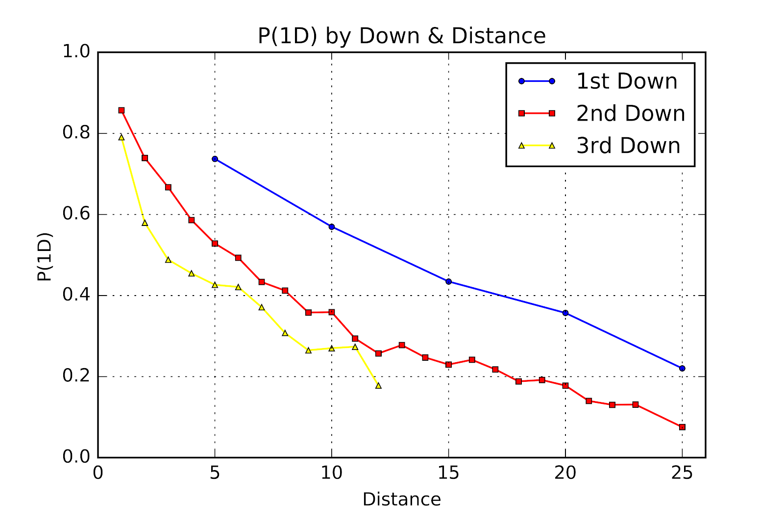

Figure 1 First Down Probability by Down & Distance

As a first-order sanity check we see that for the same distance P(1D) is higher for 1st down than for 2nd down, and for 2nd down over 3rd down. We can also see that, with limited exception, P(1D) decreases with increasing distance to gain. When we compare this graph to the existing corpus for American football we might expect Canadian 1st, 2nd, and 3rd down to look like American 2nd, 3rd, and 4th down, respectively. American football shows linear correlations between P(1D) and distance for all downs, but Figure 1 clearly contradicts that pattern. While 1st down is linear, 2nd and 3rd downs are clearly not. As to the exact values of each point in Figure 1, they are given in Table 2. The data points where N<100 have been omitted for clarity.

Distance	1st Down	2nd Down	3rd Down
1		0.8571	0.7908
2		0.7394	0.5797
3		0.6672	0.4885
4		0.5862	0.4548
5	0.7372	0.5284	0.4264
6		0.4933	0.4211
7		0.4334	0.3713
8		0.4122	0.3077
9		0.3581	0.2649
10	0.5698	0.3589	0.2701
11		0.2940	0.2737
12		0.2571
13		0.2777
14		0.2472
15	0.4346	0.2296
16		0.2415
17		0.2177
18		0.1882
19		0.1916
20	0.3570	0.1778
21		0.1399
22		0.1304
23		0.1310
24
25	0.2203	0.0754	0.0769

Table 2 First Down Probability by Down & Distance

P(1D) of 1st & 10 is 0.5841, while the P(1D) of 1st & 10 in American football is 0.6708 and for 2nd & 10 is 0.5332. 3rd & 1 in U Sports is 0.7921, 4th & 1 in the NFL is 0.6862 (Schechtman-Rook 2014). Obviously the 1-yard neutral zone is a huge factor in short yardage. P(1D) of Canadian football cannot be considered as a variation of American football, it demands its own study.

i-1st Down

As seen in Figure 1 above, P(1D) of 1st down seems to follow a linear trend. To test this a linear regression function was fitted to the 1st down data and shown in Figure 2. Confidence intervals at the 95% level are also included to give a measure of the uncertainty. The data from which Figure 2 is derived is given in Table 3

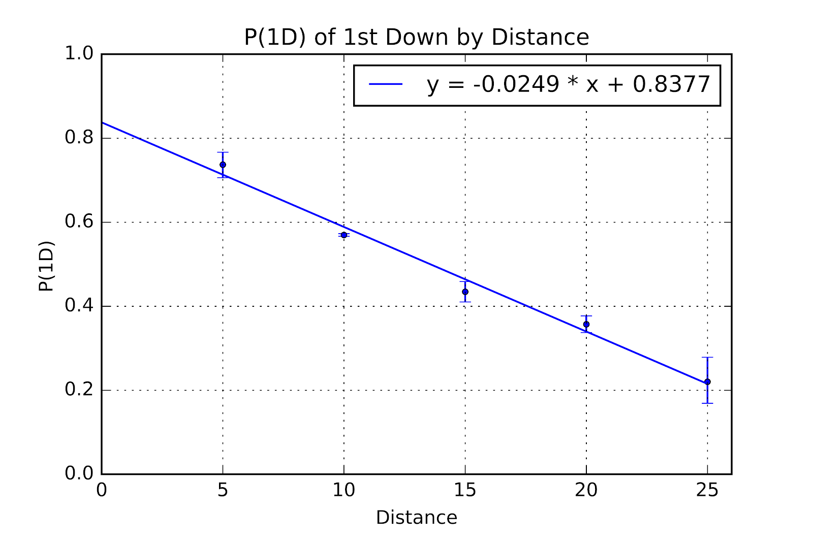Figure 2 First Down Probability, 1st Down, with Error Bars and Regression Line

Distance	Lower CL	P(1D)	Upper CL
5	0.7059	0.7372	0.7667
10	0.5667	0.5698	0.5729
15	0.4104	0.4346	0.4591
20	0.3373	0.3570	0.3770
25	0.1692	0.2203	0.2787

Table 3 P(1D) for 1st Down with 95% Confidence Intervals

The R2 value of the fitted function is 0.9865, and the RMSE is 0.0206, while RMSE/µ being 0.0445. The line does not pass through the confidence interval for 1st & 10, but this is the most common down & distance pairing by a factor of nearly 6 over the second-place combination, so this is unsurprising. The confidence interval is less than two-thirds of a percentage point. Furthermore, the line is illustrative of the trend, but not meant to show an actual physical relationship between the two. P(1D) decreases linearly with increasing distance, but this is not a physical law obliging it to be so.

With this linear trend, we can say that the marginal value of a yard on 1st down is 2.5 percentage points of P(1D). This trend breaks down at shorter distances. We should, if we idealize the game, see the trendline have a y-intercept of 1, since if the offense had 0 yards to gain they would have a 1st down, by definition. Instead the y-intercept is at 0.8377. Given that 1st down plays are almost always given in multiples of five, with no N values greater than 37 for any other distances, and that the existing trendline adequately describes the five data points given in Figure 2, this matter can be safely set aside for the moment.

ii-2nd Down

From Figure 1 we see that 2nd down breaks with tradition and is decidedly non-linear. A number of different families of functions were considered before choosing to use an exponential function. As was seen for 1st down, Figure 3 shows the 95% confidence interval for 2nd down plotted against the fitted curve, while the data is also shown in tabular form in Table 4.

Figure 3 First Down Probability, 2nd Down, with Error Bars and Regression Line

Distance	Lower CL	P(1D)	Upper CL
1	0.8460	0.8571	0.8676
2	0.7249	0.7394	0.7535
3	0.6525	0.6672	0.6818
4	0.5718	0.5862	0.6005
5	0.5153	0.5284	0.5415
6	0.4799	0.4933	0.5068
7	0.4202	0.4334	0.4467
8	0.3986	0.4122	0.4260
9	0.3433	0.3581	0.3731
10	0.3519	0.3589	0.3659
11	0.2764	0.2940	0.3122
12	0.2372	0.2571	0.2776
13	0.2536	0.2777	0.3029
14	0.2203	0.2472	0.2756
15	0.2085	0.2296	0.2518
16	0.2104	0.2415	0.2748
17	0.1856	0.2177	0.2525
18	0.1539	0.1882	0.2264
19	0.1533	0.1916	0.2348
20	0.1546	0.1778	0.2028
21	0.0989	0.1399	0.1900
22	0.0854	0.1304	0.1878
23	0.0808	0.1310	0.1970
25	0.0460	0.0754	0.1152

Table 4 P(1D) for 2nd Down with 95% Confidence Intervals

As with the 1st down graph in Figure 2, the only point where the fitted curve does not fall into the confidence interval is 2nd & 10. First, there are 24 points in this graph, and so one point not fitting into a 95% confidence interval is to be expected. Second, there are possible football reasons behind this anomaly.

Note that the point for 2nd & 10 is above the curve. Its immediate neighbours, 2nd & 9, 2nd & 11, 2nd & 12, are below the curve. These are 2nd & long plays, the result of an unsuccessful 1st down play. Bad teams have more unsuccessful plays on 1st & 10, leading to 2nd & long. But while good teams avoid losses and small gains, they are still subject to incomplete passes on 1st down. Ergo 2nd & 10 may feature an overrepresentation of good teams relative to its neighbours.

That not every point is the product of a truly random sampling of all teams is unfortunate, but known. 2nd & 1 is the product of a successful 1st & 10 play, and so should show more good teams. In applications this will have to be considered and necessary adjustments made.

Data for 2nd & 24 is not included as it only had n=97, falling just shy of the threshold of 100 that was established earlier. Large losses are uncommon, becoming rarer as the magnitude of the loss increases. Additionally, 2nd & 24 may see itself rounded to 2nd & 25, as evidence exists that referees and scorekeepers are biased toward round numbers (Burke 2008). The addition of one or two more seasons of data will push 2nd & 24 over the n=100 threshold.

As to the fitted function itself, most regression wizards only use the form y=aebx, which only allows the function to be stretched as well as translated horizontally. This means the the horizontal asymptote is always at 0. Using a solver through the formy=aebx+callowed for the function to be translated vertically, giving a far better fit to the data. While R2 for nonlinear functions must be treated with skepticism, it is measured at 0.9910 for this data, while the RMSE is 0.0194 and the RMSE/µ is 0.0565

Since the second parameter of the fitted function is negative, the function is an exponential decay function. This breaks from what we have seen in 1st down and in American football. We might posit that the effect of the one-yard neutral zone, which provides a massive advantage to the offense in short yardage, slowly diminishes with increasing distance, and leaves a linear model underneath. It seems implausible, however, that th impact of the neutral zone is still being felt 10-12 yards from the line to gain.

An important feature of exponential decay functions is that they have asymptotes. As distances increases P(1D) will continue to decrease in smaller and smaller amounts but will eventually approach, yet never reach, its asymptote. For the 2nd down fitted function this asymptote is at 0.0791. While intuitively we know that P(1D) can never truly be 0, it should at least become vanishingly small. Instead this model, and the data behind it, implies that P(1D) has a lower limit of about 8%. One way that a team could get convert an incredibly long distance would be for the defence to commit a penalty, especially one that provides an automatic first down. Indeed, of the 353 plays in the data of 2nd & 26+, there were 34 successful cases(9.63%). Of these, 12 had defensive penalties bring about first downs (35.29%), and in one bizarre case the defense intercepted a pass but the quarterback forced a fumble that was recovered by the offense for a first down. That the lower bound of P(1D) at extreme distances is driven by the inability of the defence to not commit major penalties gives a name to this phenomenon: The Stupidity Asymptote. The hypothesis of the Stupidity Asymptote for large distances-to-gain is as follows:

P(1D) is asymptotic as distance-to-gain increases
This asymptote is much higher than would be expected
This asymptote is driven by defensive penalties awarding automatic first downs

While some penalties are inevitable, and a few others may even be desirable, penalties such as roughing the passer are inexcusable and create the narrative of the Stupidity Asymptote. In applied terms the Stupidity Asymptote may prove useful to an offense in a very long-yardage situation, knowing that P(1D) is lower-bound they can extrapolate beyond the available data, and may even make playcalls aimed at improving the chances of getting such a penalty called against the defense. Defensively there should be an emphasis in certain situations to avoid any risk of such a penalty. While the idea of avoiding a penalty that would give the offense an automatic first down is hardly revolutionary we now have evidence describing the scope of the problem, of how often defenses self-destruct.

Unlike 1st down, which is dominated by 1st & 10 and the other points are the result of penalties, 2nd down is the result of the preceding 1st down. Therefore the shorter distances, being the result of more successful plays on 1st & 10, tend to be overrepresented by better teams, and inflate the P(1D) of the “average” team. Conversely, as distance-to-gain increases we will see an overrepresentation of bad teams, understating P(1D) of the average team.

One will note that 2nd & 10 is noticeably above the fitted curve, standing in contrast to the points around it that hew to the line. If we consider how 2nd down plays and their distances come about we can consider that 2nd & 10 is the result of no gain on 1st & 10, while the points around it are the result of a small gain or loss. Plays with no gain are most commonly the result of incomplete passes, while small gains and losses come from unsuccessful runs. Both good and bad teams will have incomplete passes on 1st & 10, but bad teams are much more likely to have an unsuccessful run. Ergo, the P(1D) of 2nd & 10 will be higher by dint of having more good teams among its ranks, relative to its neighbours.

Classification of football plays as being “successful” or “unsuccessful” is fraught with difficulties, as football plays are very context-dependent. P(1D) offers a more objective, if not entirely complete, answer to that question. We can consider a play to be successful in terms of P(1D) if the play either gains a first down or results in a higher P(1D) for the next play. Since P(1D) of 1st & 10 is 0.5698, then we can look at our table of P(1D) for 2nd down and see that P(1D) of 2nd & 5 is 0.5284, not quite good enough, while P(1D) of 2nd & 4 is 0.5862. Thus we can say that a 1st & 10 play must gain 6 yards to be considered “successful” in terms of P(1D). Similar logic can be applied for all other downs and distances.

iii-3rd Down

Discussion of 3rd down is, to some extent, confounded by the circumstances which dominate 3rd down conversion attempts. While all teams regularly make 3rd & 1 attempts, longer 3rd & 1 is usually the result of teams acting out of necessity or desperation, these being bad teams. Thus, we can probably assume that 3rd down P(1D) is consistently underestimated. 3rd down, and its attendant error, are shown graphically in Figure 4 and in tabular form in Table 5.

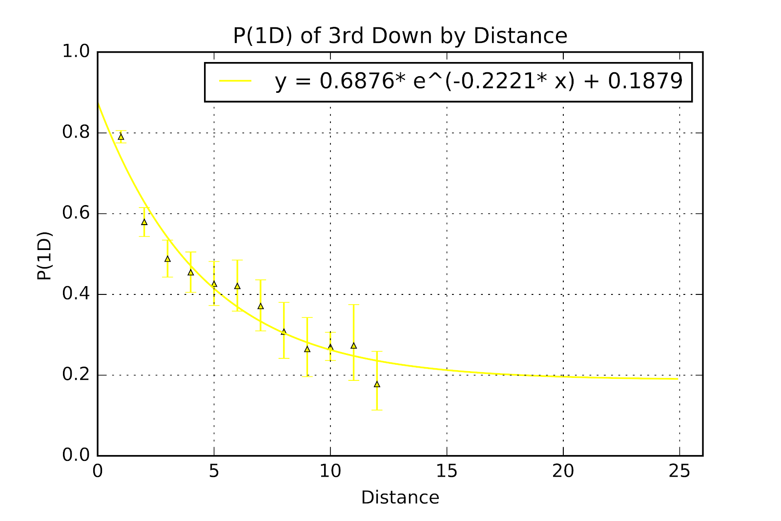
Figure 4 First Down Probability, 3rd Down, with Error Bars and Regression Line

Distance	Lower CL	P(1D)	Upper CL
1	0.7753	0.7908	0.8058
2	0.5437	0.5797	0.6151
3	0.4428	0.4885	0.5343
4	0.4051	0.4548	0.5051
5	0.3727	0.4264	0.4815
6	0.3587	0.4211	0.4853
7	0.3096	0.3713	0.4362
8	0.2415	0.3077	0.3802
9	0.1965	0.2649	0.3428
10	0.2362	0.2701	0.3060
11	0.1872	0.2737	0.3748
12	0.1137	0.1780	0.2591

Table 5 P(1D) for 3rd Down with 95% Confidence Intervals

Similar in appearance to 2nd down, 3rd down also fit an exponential decay curve of the form y=aebx+c, although with RMSE of 0.0374, RMSE/µ of 0.0930 and a R2 of 0.9452. Given the relative shortage of data these are obviously much rougher numbers than for 2nd down, but some conclusions can still be drawn. The fitted curve still shows an asymptote, however this asymptote is much higher than for 2nd down. Given the very wide confidence intervals for 3rd & 11 and 3rd & 12, and the complete lack of any points beyond this, we feel that this is probably more an artefact of insufficient data than a true representation of the asymptote.

When compared with Bell (1982) these values for P(1D) on 3rd down are not well correlated. Whether due to the passing of time or Bell’s limited data set, or his use of CFL data will remain an unanswered question for the time being, but his values, both raw and smoothed, consistently fail to fit into the confidence intervals listed above.

The particular case of 3rd & 1 merits further discussion. With a P(1D) of 0.7903 the play is a good bet, but not a sure one. Of the 3295 instances of 3rd & 1 attempts there were 764 failures (23.19%). But of these failures there were offensive penalties on 152 of them (19.90%). A full fifth of failures driven by offensive penalties. The nature of the type of wedge or sneak play generally run on 3rd & 1 limits the scope of penalties that are plausible, the penalties in these situations are generally procedural and avoidable. A review of some game film shows that the penalties are often called against players such as receivers, who are not even involved in the play. This may be seen as the analogue to the Stupidity Asymptote, perhaps the “Stupidity Ceiling.” Unlike the Stupidity Asymptote, the Stupidity Ceiling is much more fixable, as the penalties do not arise from play. The key recommendations are:

Not to waggle the receivers. Since the receivers are, at best, an afterthought, and any pass plays are akin to a trick play, the benefit of the waggle is negligible and it often results in a penalty.
Not to alter the snap count. There is a general temptation to use a hard count in an effort to draw the defense offsides. Video analysis shows that this is, ironically, a frequent cause of offensive penalties.

Just as a 1st & 10 play can be considered a success if it gains 6 yards or more, because it results in a higher P(1D) than the preceding play, 2nd downs can also be evaluated along similar lines. If an offense does gain 6 yards o 1st & 10, they face 2nd & 4. With a P(1D) of 0.5862 they would have to gain 3 yards to create 3rd & 1 in order for the play to be considered “successful.” Of course, this is not an entirely complete method of assessing a play’s utility, as a 3rd & 1 play may still end a drive. If the field position is poor it may be better to punt, as even with a high probability of converting the consequences of failing to convert may outweigh the benefits of succeeding. Sti8ll, P(1D) provides a first-order means of sorting plays in an objective manner.

iv-& Goal

Because of the compression effects of the end zone P(1D) for & Goal situations cannot be included in tables for P(1D) in other situations. In addition to the field becoming compressed by the back of the end zone, there are marked changes in both offensive and defensive strategies. Figure 5 and Table 6 show P(1D) for & Goal situations.

Figure 5 P(1D) by Down & Distance for & Goal

Distance	1st Down	2nd Down	3rd Down
1	0.9010	0.8563	0.7043
2	0.8821	0.7769
3	0.8552	0.6711
4	0.8115	0.6000
5	0.7441	0.4697
6	0.7329	0.5648
7	0.6757	0.4620
8	0.6659	0.4000
9	0.6291	0.4179
10	0.5725	0.4464

Table 6 P(1D) by Down & Distance for & Goal

Unsurprisingly, there are no data points of distance greater than 10. In order to be & Goal the 1st down has to occur within the 10-yard line, so for a play to be 1st & goal behind the 10 it requires a penalty to push the offense backwards. On 2nd or 3rd down it would require a loss on a previous down. These are all rare enough cases that none reach the 100-instance threshold.

1st & Goal from the 1 is the highest point for P(1D) that we see in any situation, unsurprisingly. It is also a frequently occuring state (n=818), because a number of defensive penalties will cause a 1st down at the 1-yard line. In general the same advice from the discussion of 3rd & 1 earlier holds here.

The 2nd down data shows an odd jump, where 2nd & 5 has a much lower P(1D) than 2nd & 6. A look at Table 7 shows that all the points are well-populated, 2nd & 5 even more so than the adjacent points. If we compare this to 1st down we also see more data points at 1st & 5 than 1st & 4 or 1st & 6, and we see that the resultant value is less than we might expect. The most plausible explanation may come to the way in which coaches gameplan. For reasons of practicality coaches group different distances together as being the same basic scenario. Using the 5-yard line as one of these cutoffs is common, and often represents where an offense shifts from “red zone” to “goal line” in its mode of thinking. In doing so teams will change their playcalling and also often drastically change their personnel, substituting for larger players and adopting a compressed formation. It may well be that this shift is premature at the 5-yard line, and that coaches are consistently overestimating the ability of their goal line offense to gain 5 yards., whereas at the 6 they are using their red zone offense, usually a subset of their base offense. A detailed film review is necessary to corroborate or disprove this notion.

Distance	1st Down	2nd Down	3rd Down
1	813	484	234
2	405	260	84
3	365	226
4	368	216
5	512	270
6	461	196
7	415	176
8	419	145
9	406	137
10	495	158

Table 7 Sample sizes for & Goal situations

4-Conclusion

Insofar as the development of P(1D) is concerned, the development of methods to make team-specific adjustments is a possible area of future research, but it would be difficult to develop a model with good confidence during the season. A first approximation would be to use a team’s P(1D) at 1st & 10 to adjust P(1D) at other downs & distances, though this would require showing that P(1D) is correlated across states for a given team.

With the advancement of a first understanding of P(1D) in Canadian football the door is opened to further exploration in the field. Using methods already developed for American football the pace of development can be much faster, in spite of the comparatively limited resources available. Expected Points, Win Probability and examination of kicking metrics are the logical areas of future research. An improved understanding of the nature of Canadian football will lead to more informed strategic decisions, either validating current approaches or introducing new ones.