1 – Abstract

An examination of the existing scholarship of First Down Probability (P(1D)) in American football. A fairly unambiguous question, this work reviews ten studies over the past 45 years, albeit mostly in the last decade. Results are generally consistent across sources that P(1D) decreases in linear proportion to distance-to-gain for 1st and 2nd downs, while different sources model 3rd down as being either a weakly fit linear relationship or a slight exponential fit.

4th down was not examined fully by any source because of insufficient data. What data points can be confidently placed seem very close to 3rd down, leading to discussion over whether 3rd down data can serve as a proxy for 4th down in decision-making models.

2 – Introduction

At the outset, this article was intended as the literature review section for a separate study of P(1D). Eventually the literature review overtook the paper and became its own work. The growth in football analytics in recent years means that what once would have merited a paragraph or two now requires several pages. There are countless blogs, university courses (Lopez 2016), academic journals (IOS Press n.d.; “MIT Sloan Sports Analytics Conference” n.d.) and major conferences (Glickman n.d.) dedicated to the topic. As the field grows, the question of what constitutes football analytics has been raised. While lacking a fixed definition, the idea of searching for predictive models meaningful to the business of winning games is a reasonable starting point (Burke 2014). This demands both sufficient understanding of football to know which questions to ask, and sufficient understanding of mathematics to answer those questions. Critically, the ability to communicate those answers cannot be neglected (Causey 2015). The rise in capability and availability of computers has dramatically changed the landscape of quantitative analysis, recording ever more granular data (Cochran 2011). There exists an arms race between our ability to collect data and our ability to process it (Alamar and Mehrotra 2011). The amateur football analyst now has access to more data than any professional researcher could have dreamed of 20 years ago (Horowitz 2016). Indeed, there is something of a cottage industry in providing NFL play-by-play data for the hobbyist (Myers 2011).

Among the first metrics derived from this data was First Down Probability, the likelihood that a team will convert a first down from a given down and distance. It is the probability of converting within the entire drive, and not merely on the play in question. For example, if a team gains 5 yards on 1st & 10 to face 2nd & 5, followed by a 7-yard gain resulting in a new 1st & 10, the original 1st & 10 play is considered to have led to a successful conversion, even if the conversion did not happen on that play. Touchdowns are also considered successful conversions, for obvious reasons. P(1D) permits plays to be assessed as successes or failures, based on whether the net P(1D) is positive, and allows for more informed decision-making.

3 – First Down Probability

Conventional football wisdom holds that 1st & 10 plays should gain 4 yards in order to be considered successful. 2nd down plays should gain half of the remaining yardage, to wit, 2nd & 6 should look to gain 3 yards. 3rd down plays are expected to gain all of the remaining yardage, as conventional wisdom invariably kicks on 4th down. A team facing 2nd & 6 or fewer, or 3rd & 3 or fewer, is said to be “on schedule.” This approach was codified in the seminal 1988 work in football analysis, The Hidden Game of Football (Carroll et al. 1998).

The first published attempt to quantify a team’s probability of converting a given down and distance is likely the work of Carter & Machol (Carter and Machol 1971; 1978). Virgil Carter, quarterback of the Cincinnati Bengals doing graduate work in the offseason, used play-by-play data from the 1969 NFL season (n=8,373) to create an elementary EP. He and Machol expanded on this work significantly, with an eye to influencing 4th down decisions. In order to do so he created a very limited P(1D) study of the 1971 NFL season, covering only 4th down situations with distances to gain of 5 yards or fewer, which has been reproduced in Table 1 (Carter and Machol 1978). However, Carter & Machol’s work was not intended to be a P(1D) study; it was simply necessary to achieve the aims of their paper. It was clearly meant as an approximate method; it uses a different, and much smaller, data set than any of the other work in either paper (Carter and Machol 1971), and it is quite likely that neither author concerned himself with the broader value that a P(1D) study could bring. Indeed, with the technology of the era, it would have been impossible to do a full examination of P(1D).

Distance	n	Successes	P(1D)	σ
1	543	388	0.715	0.019
2	327	186	0.569	0.027
3	356	146	0.410	0.026
4	302	97	0.322	0.027
5	336	91	0.271	0.024

Table 1 First Down Probabilities for 3rd Down by Distance (Carter and Machol 1978)

While studying Expected Points (EP) and 4th down decision-making, Wright (Wright 2007) looked at P(1D) of five NFL teams in the 2005 season. This work, albeit limited in scope, chose five teams that were deemed to represent a cross-section of strengths and weaknesses. 3rd and 4th down attempts were combined to better populate the dataset for each team, necessary because of the use of only one season and one team at a time. While the results are noisy for want of data, Wright used logistic regression rather than fitting a function to the aggregate points. The resultant fits are close to linear for four of the five teams but each team has too few data points to consider them as a meaningful assessment of P(1D) in toto, but the results are reconcilable with future work in the field.

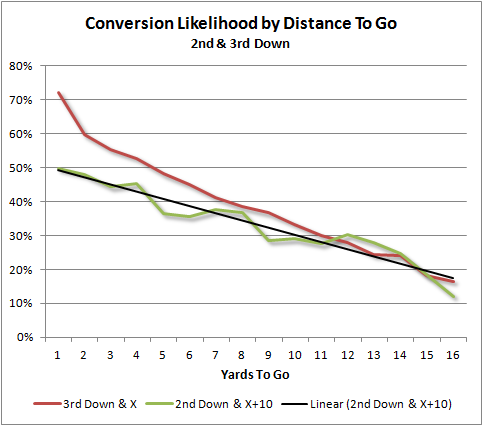
After decades of dormancy, Burke (2008) developed a complete model of P(1D) across all downs and distances. Burke’s results for 2nd and 3rd down P(1D) are included in Figure 1 and they show a linear trend for P(1D) on both 2nd and 3rd down, (1st down is omitted because of the paucity of non-1st & 10 plays). 3rd & 1 is a noticeable outlier from the rest of the 3rd down trend, which can be explained by the caprices of football record-keeping. Any measurement of less than 1 yard to gain is recorded as 3rd & 1, and so will include many “3rd & inches” situations. While the “inches” notation is common in television broadcasts to illustrate the situation to the viewer, official records do not include it. While all distance measurements include a range of distances that are all rounded to a whole number, the magnitude of this effect is only noteworthy for “& 1” situations, where the range spans from a fraction of an inch to 54”.

Figure 1 P(1D) for 2nd and 3rd Down by Distance (Burke 2013)

Owing to the relative scarcity of fourth down attempts, Krasker (2010) examined whether 4th down data could be augmented with 3rd down data, concluding that it could not. However, Krasker’s argument was based on optimal decision-making. Given various arguments that NFL decisions are sub-optimal (Romer 2006; Gallagher 2011; Stuart 2012) and that coaches rarely consider 4th down conversion attempt, the usefulness of 3rd down data as a reasonable approximation of 4th down may still be appropriate.

As part of an analysis of NFL decision-making, Gallagher (2011) examined P(1D) of 3rd down across a range of distances to gain. Contrary to Krasker’s indications, Gallagher used these as a proxy for 4th down conversion rates. Gallagher’s results are consistent with Burke’s (Burke 2008) linear trend, as well as the discontinuity at 3rd & 1.

Moving beyond linear models, Cafarelli, Rigdon, & Rigdon (2012) fitted logistic regression functions to assess 3rd down conversion rates across the NFL and for individual teams. While previous works have all focused on linear models, the statistical methods here are more sophisticated. Linear models provide a good fit over those distances to gain for which we have ample data, but imply that P(1D) will reach 0 somewhere around 3rd & 30, and be negative thereafter. This restricts the viability of those models when discussing very long distances, a problem avoided by using logistic regression.

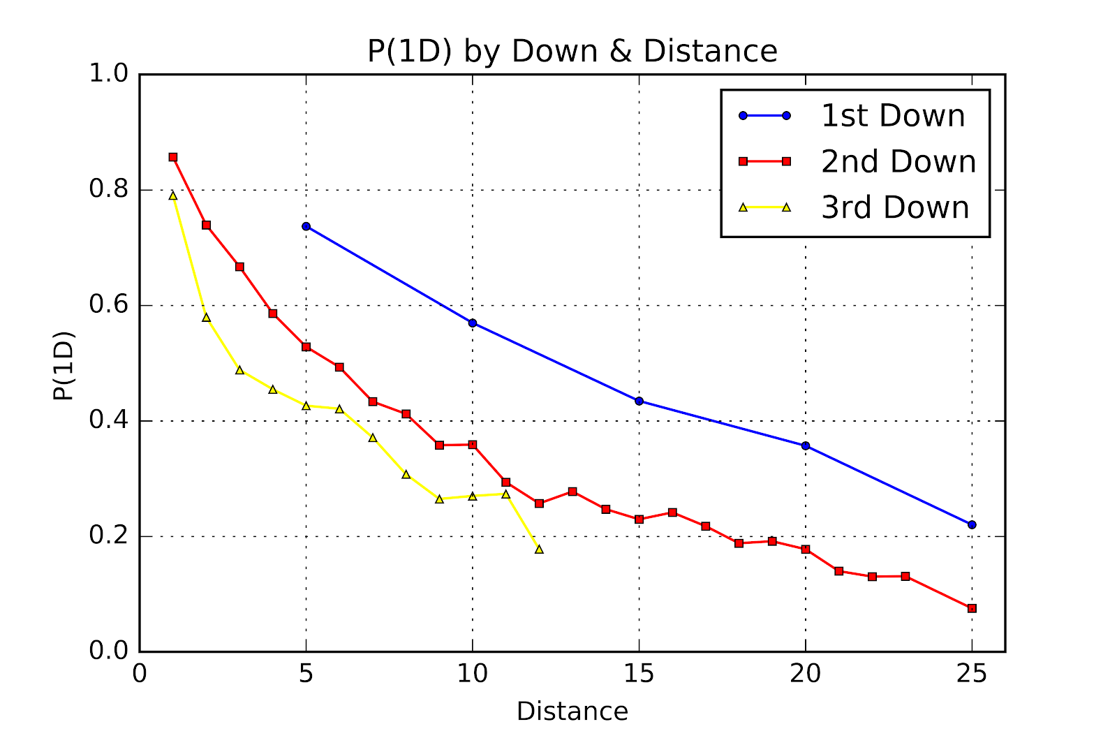
Andrew Schechtman-Rook (2014b) of PhD Football reproduced Burke’s (2008) earlier work, using a data set of all plays from 2000-2011 (nearly 3000 games and a total of 262,601 plays) to develop his results and arriving at generally similar conclusions. Schechtman-Rook compares his work, shown in Figure 2, to Burke (2008), and finds the results, in his own words, “copacetic” (Schechtman-Rook 2014b). 2nd down P(1D) is about 15 percentage points less than P(1D) for 1st down at the same distance, and 3rd down is worth 20 percentage points less than the equivalent 2nd down. Only 1 and 2-yard distances were considered for 4th down. These results are included in Figure 2, and the numerical results in Table 2 (Schechtman-Rook 2014a).

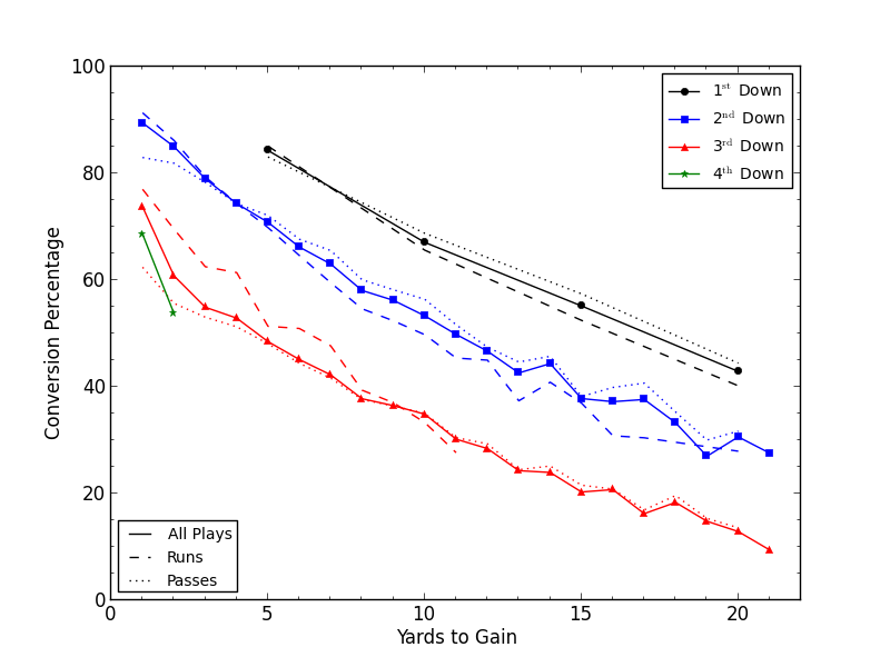https://blogger.googleusercontent.com/img/b/R29vZ2xl/AVvXsEgkw0VHxIlQiXQncEpzA6vgjkgJghvKNe9OLwTi6fWq9BnRUvbZirB3t_s8Px4Ie7i2kxcxGy_9dkgtiVewZNC5AfPEpAqMJoCG6RR4k0iB81C4FOS01jnzvVJX24Fq3pUAjnvzUWO66sCE/s1600/firstdownlikelihood_all.png

Figure 2 First Down Probability by Down and Distance (Schechtman-Rook 2014b)

	1	2	3	4
1	-	89.47	73.74	68.62
2	-	85.03	60.82	53.77
3	-	79.01	54.92	-
4	-	74.35	52.89	-
5	84.30	70.84	48.48	-
6	-	66.21	45.13	-
7	-	63.02	42.25	-
8	-	58.06	37.77	-
9	-	56.22	36.48	-
10	67.08	53.32	34.88	-
11	-	49.84	30.20	-
12	-	46.69	28.44	-
13	-	42.61	24.29	-
14	-	44.36	23.96	-
15	55.16	37.81	20.30	-
16	-	37.22	20.74	-
17	-	37.64	16.24	-
18	-	33.28	18.34	-
19	-	27.00	14.81	-
20	42.89	30.62	12.88	-
21	-	27.59	09.43	-

Table 2 P(1D) By Down and Distance (Schechtman-Rook 2014a)

When compared to Carter & Machol’s (1978) results shown in Table 1 the differences are startling. P(1D) on 3rd down is 2-30 percentage points better in 2014 than it was in 1971, a testament to the evolution of the game in all its facets. Comparing Schechtman-Rook’s results to Burke’s(2013) we see a much closer match. Although Burke’s numerical results are not available a visual comparison of Burke’s graph to Schechtman-Rook’s results show a fair match. Of note is the discontinuity at 3rd & 1 relative to the otherwise linear trend from 3rd & 2 to 3rd & 20. Both have slopes of approximately -0.03 from distances of 2 to 15.

Schechtman-Rook (2014b) goes into further analysis by splitting passing and rushing plays. Consistent with other authors in the field (Alamar 2010; Schatz 2004; Stuart 2008), passing plays result in a higher P(1D) than rushing plays for 1st downs of greater than 5 yards, 2nd downs greater than 2 yards, and 3rd downs greater than 8 yards. However, NFL record-keeping shows sacks as being pass plays and QB scrambles for positive gains as rushing plays. Therefore, a number of plays intended as passes are being recorded as rushes, but only those where yardage was gained, tending to benefit the consideration of rushing plays (Schechtman-Rook 2014b). This curiosity was then analyzed in greater detail by removing all rushing plays where the rusher was a quarterback. This adjustment shows that rushing is only favourable on 3rd downs of less than 4 yards. The implication here is that a great deal of QB scrambles on 3rd downs lead to first downs (Schechtman-Rook 2014b).

Marking the first foray into college football P(1D) analysis, Anthony Santana (2010) developed a P(1D) model from college football data, using over 105,000 plays where both teams were members of BCS conferences. He used exponential regression for all downs. Whether these fits are more appropriate than the linear fits seen elsewhere is an area of potential research. His results are included in Figure 3 (Santana 2010). Santana set his y-intercept at 1 for both 1st and 2nd downs, but found that fixing this intercept resulted in problems for the 3rd down curve. He posits that this may be due to error in spotting the ball (Santana 2010).

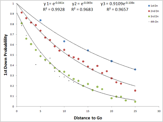
Figure 3 P(1D) by Down and Distance (Santana 2010)

Why college football data would fit exponential curves as opposed to the linear results from NFL data remains an open question. With the large dataset it seems improbable that this is the result of random error in the sample and raises the question of whether there is a particular reason that college football would show different properties from NFL football. Santana’s (2010) work shows no meaningful difference between 3rd and 4th down data points at the same distance, and in his conclusions, he encourages using 3rd down data as a proxy in 4th down decision-making.

Mills (2013) looked at P(1D) on third down. As with the results of Burke (2008) and others working on NFL data, the college football data shows a spike at 3rd & 1 and linear trend thereafter. Mills compared five consecutive seasons of data from 2008-2012, copied in Figure 4, and found no meaningful difference across seasons. A quantitative comparison against other NFL works shows that college P(1D) is roughly equal to NFL P(1D) on 3rd and 1 but lags at longer distances. We might suggest that his is due to more prolific and sophisticated NFL passing attacks, as well as differences in rules and applications of said rules in the NFL that frequently provide first-down-granting penalties to the offense. That Mills work would parallel NFL studies so well casts some doubt on Santana’s (2010) exponential fits.

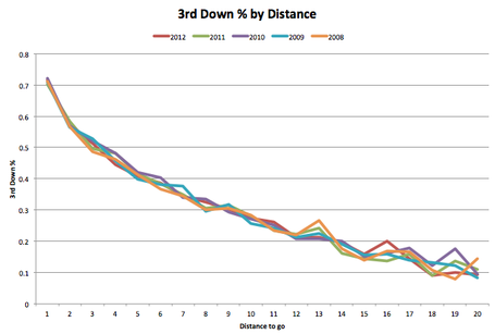Figure 4 P(1D) for NCAA on 3rd Down (Mills 2013)

More research on P(1D) in college football was done by the sports research group Stats Insights (Feinstein 2014). While the results of their work are not meaningfully different from other efforts, their discussion makes several salient points. Primarily, they argue that average 1st down gain is a more effective measure of offensive success than 3rd down conversion rates. The ability to convert a given 3rd down is, obviously, dependent on the distance to gain. This distance is the result of success on previous downs. Average gain on 1st down allows for consideration of the magnitude of gains. A 4o yard gain is more than just a first down, it also obviates the need to gain two or three more first downs while driving for a touchdown.

A third group, the founders of the Minitab statistical software, created a P(1D) model of college football using data from 2006-2011, separated by &-Goal and non-&-Goal situations (Rudy 2015). Rudy’s results, attached in Figure 5, emerge about 10-15 percentage points lower than Santana (2010), perhaps because of Santana’s choice to only consider only games between BCS-level opponents.

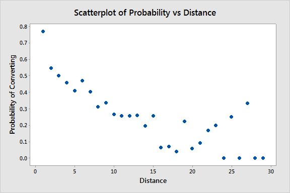
Figure 5 P(1D) for 3rd Down by Distance (Rudy, 2015b)

Rudy’s results also show an enormous amount of noise, and without the disclosure of n values or error bars it becomes difficult to place faith in the these results since they seem to show much more noise than any of the other studies. Indeed, between 3rd & 24 and 3rd & 30 we see P(1D) vary between 0 and about 0.35. These are almost certainly the result of small samples, especially for distances that are not multiples of 5.

4 – Conclusion

P(1D) is not inherently useful in its own right for making in-game decisions, save for occasional situations involving accepting penalties (Burke 2013), but it is an absolutely critical part of almost all decision models. P(1D) of 4th down is particularly important, as it is a driver of 4th down decision-making, which is the largest area of study in modern football analytics.

P(1D) is likely a mature field, and we can expect future developments to be incremental. The large datasets currently available leave little room or need for advanced statistical techniques as each data point has negligible error. Further approaches may investigate whether teams show unique P(1D) functions, although Cafarelli et al. (2012) seem to indicate otherwise. The historiography of P(1D) may be worth investigating, particularly as game decisions slowly move towards a greater use of 4th down, since this will necessarily increase P(1D) across the first three downs. Although it is likely that opposing defenses will identify these tendencies fairly quickly and seek to mitigate them, there are still benefits to be gained from finding an equilibrium. As more data becomes available we may also see development in data selection; whether to include data from late-game situations or large score differentials. Presently such distinctions are based on heuristic intuition but more objective methods maybe forthcoming in the field.