Passes and Patterns: It’s Spelt “Rouge:” Expected Points in U Sports

1. Abstract

For an existing database of U Sports play-by-play data five different models were created to look at Expected Points in U Sports football. The results of these models are presented, in addition to the results of the raw data, allowing the models to be compared to the raw data and against one another. Furthermore, extensive correlation graphs are presented to allow models to be assessed based on their effectiveness in predicting EP. The multi-layer perceptron model proves itself to be the most effective across all scenarios, followed by the gradient boosting and k-nearest neighbours models. The random forest and logistic regression models proved poor estimators of EP and are contraindicated for future use.

2. Introduction

Having already firmly established the state of the art of football analytics (Clement 2018c, [b] 2018, [a] 2018), and begun a modest foray into the presentation of original findings (Clement 2018d, [e] 2018), the examination of Expected Points (EP) and modelizations of EP are a natural progression. While there currently exists one known effort to develop a U Sports EP model (Taylor 2013), the methodology behind this is unknown. There is also an EP model, based on logistic regression, folded into an existing CFL Win Probability (WP) model (Thiel 2019).

Although the determination of EP values for various scenarios is of value, the greater goal is to be able to extrapolate from the existing data to accurately assess the EP value of plays that are not so common as to be able to be determined directly. These cases require statistical models. Five models were chosen to examine, chosen to represent a broad spectrum of different approaches that are appropriate to the multiclass nature of the problem. The intent is to develop a response model of EP, one that carries forward until the next scoring play, or end of half, as opposed to a raw EP model, which only looks within a drive. Response models are generally more applicable because they can consider downstream effects such as field position, and the impact of poor field position on the opposing team’s scoring chances should the current drive fail to score.

3. Methods

Data from the existing Passes and Patterns U Sports database was used in creating this EP database (Clement 2018f). Following with the object-oriented approach for the parsing of the data, additional objects were created to describe a number of situations for which EP would need to be treated separately.

An EP object was first created for kickoffs (class KO), field goals (class FG), and punts (class Punt). An array was created for each of these classes to store 110 instances, one for each yard of the field.

While the nominal value of scoring plays is well understood - touchdowns are worth six points plus their conversion values, field goals are three points, and so on, the true value of a scoring play must also consider the aftermath, wherein the ball is returned to the opponent, and the EP of that possession. This effect must be folded into the value of the scoring play.

In order to develop this calculation, an additional object class was created to hold EP values for all situations of down, distance, and field position (class EP). A 3-dimensional list 4 x 26 x 110 held instances of this object. Each object has an attribute to count the incidence of each EP_INPUT for plays of that down, distance and field position. The EP value could then be determined by multiplying the number of instances of each outcome by the score value of that outcome, and dividing by the total number of instances.

Each field goal object in the array looped through the database and counted the number of field goal attempts from that field position, and the trinary outcome as GOOD, MISSED, or ROUGE. The probabilities of each outcome were then determined. The EP values of these field goals was not calculated initially, set aside until the score values had been defined. By convention field goals here are defined by the line of scrimmage, and so the actual distance of the kick is some 7 yards further than the listed field position, given the snap and hold.

KO objects initially calculated the EP value of a kickoff by directly determining the EP value of the kick from its EP_INPUT attributes, much as the EP objects are calculated. However, this was found to give a large positive EP value to kickoffs, since teams who score touchdowns tend to be the better teams, and those teams tend to score repeatedly. Thus, what was being measured was that better teams are better, and tend to score more. In order to avoid this, EP was instead calculated by averaging the EP value of the subsequent scrimmage play.

Previous studies have adjusted the score values once, by subtracting the EP value of the subsequent kickoff, usually by using the average starting field position. However, doing so will cause a downstream change of all EP values as the component values that were used to calculate their EP values have changed, and when all of those have been calculated then the adjustment for the value of a kickoff will also need to be recalculated. Thus we chose to repeat this calculation iteratively in a loop until we reached convergence. Convergence was defined as when the largest percentage change for all four score values was less than 10-17. This value was chosen because at 10-18 the small vacillations cause the value for a rouge to oscillate between two values and not converge further. Any error at this point is vanishingly small. Indeed the score values converge quickly enough that after three or four loops it is beyond any reasonable expectation of precision, and it converges by about on order of magnitude per loop. The final values for all four scoring plays are given in Table 1. Note that the end of a half is always worth 0 points, and has no confidence interval because its value is defined.

Once the values of the scoring plays had converged and EP values were fixed, the 95% confidence intervals for each EP object in the EP_ARRAY by bootstrapping from the collection of EP inputs. A total of 1000 bootstrap replicates were used, well in excess of recommendations for this confidence level (Wilcox 2010; Davidson and MacKinnon 2000). Bootstrapping was the easiest method for determining variance of this kind of discrete multinomial distribution, where the alternatives were very laborious, such as one-vs-all binomial comparisons folded together. Bootstrapping is also effective for fairly small datasets. This allowed us to determine the upper and lower confidence limits for each scoring value, further elaborating Table 1.

Scoring play	Lower CL	Score value	Upper CL
Field Goal	2.9825	3.1020	3.2011
Rouge	0.9825	1.1020	1.2011
Safety	-2.7017	-2.6328	-2.5665
Touchdown	7.1480	7.1677	7.1893
Half	N/A	0	N/A

Table 1 Converged score values with upper and lower confidence intervals

The adjustment for kickoff score values was defined as 6 + P(FGGOOD(5)) + EP(KO65). This led to an unexpected discovery, that even with the new method of calculating the EP of a kickoff that removes the effect that teams kicking off are generally better, the EP value of a kickoff is still positive for the kicking team. That is, the team receiving the ball ends up, on average, in negative EP position. An obscure rule allows teams that have surrendered a touchdown the option of receiving the subsequent kickoff or kicking themselves. Receiving the kickoff is the near-universal choice, but these results imply that choosing to kick is worth about ⅓ of a point. At this time we cannot recommend taking this highly unorthodox choice until further evidence has been presented, but this is a highly counterintuitive result that merits further investigation. This option was not considered in the code but would result in touchdowns having a value of around 6.85 points

Rouges always result in the defense receiving the ball at the -35, and so the value of a rouge is 1 - EP(1&1075). Since EP(1&1075) is negative the resulting value of a rouge is slightly greater than 1.

After a field goal or a safety the defense has the option to receive the at the -35 yard line or to receive a kickoff, or to kickoff themselves. Choosing to kickoff was not included in the code as it is such a rare choice, but it was assumed that decision-making would be rational between the other two choices. After a field goal the kickoff is from the -45 yard line, and so teams are better to take the ball directly at their own 35 yard line, such that field goals are worth slightly more than 3 points.

By contrast, kickoffs after safeties are from the -35 yard line. That 10-yard difference makes forcing a kickoff the better option. In fact, that 10 yard change is enough to cause a ¾-point difference in the EP value of the kickoff.

a. Feature Selection

Data was pulled from the database by iterating over plays and game and copying the appropriate features into a Python list structure, and thereafter converted in a pandas dataframe (McKinney 2010). The pandas dataframe allows for some erasier manipulation of the data, including labelling features and converting features to categorical types without the need to manually use one-hot encoding.

i. Down

Down is included as a continuous feature. Ordinarily down should be categorical feature, since the downs are ordinal and not numerical in nature. That is, 2nd down is not “twice as much down” as 1st down. Unfortunately, sklearn has poor support for categorical data, and would require one-hot encoding through the pandas get_dummies feature (McKinney 2010). However, results with this method proved, at best, to be marginally better than when leaving down continuous, even for the models such as logistic regression and k-nearest neighbours where this might be expected to have the greatest impact. One-hot encoding also generates a risk of overfitting to the categorical feature in question, results in a massive (>50%) increase in computation time. Thus, down has been left as a simple continuous feature for expedience, an because the risks outweigh the small benefits. The down feature can be equal to 1, 2, or 3. While the database itself has some plays listed as being “0” down, to account for PAT and kickoff plays, these are not being considered in the development of these EP models.

ii. Distance

Distance to gain is a continuous numerical feature in this dataset, capable of holding any integer values from 1 to 109, inclusively, though in this case only distance values of 25 or less are considered, and values above that are quite rare. While plays with distances greater than 25 yards are included in the dataset they are not shown in the visualizations, as the region would be very sparse and would distract from the more pertinent aspects.

iii. Field Position

Field position is measured in yards from the goal line, and, like distance, can range from 1 to 109. Contrary to distance, however, the entire range of field position is seen in the database and included in the models. Certain combinations of distance and field position are not included as they are impossible. It is impossible for the line to gain to be behind the -11-yard line, as that would imply that 1st & 10 occurred within one’s own end zone, and it is impossible for the line to gain to be past the goal line, as that is the definition of an & Goal situation, and the line to gain is defined to be equal to the goal line.

b. Model Selection

While the raw EP value is a valid approach for determining the value of common situations, small sample sizes limit its effectiveness in other situations, particularly at longer distances and on later downs. Therefore a model of some kind is needed to interpolate the gaps. While originally the simplest model was applied, that of a simple weighted average of the immediate neighbours, this proved inadequate stil, as it lacked the sophistication to use more data than those in the immediate vicinity, causing sparsely populated regions to become ill-defined.

More sophisticated methods were sought, leading to the scikit-learn package (Pedregosa et al. 2011). This package offers various supervised learning models. Football scoring is, as mentioned, a discrete multinomial affair, and so the model used to represent it should be based on this multiclass structure. Therefore, rather than regression algorithms treating scoring continuously, it is preferable to model scoring categorically, and then map those categorical classification probabilities to score values to determine the EP value of a situation.

To assign scoring probabilities to plays in common situations would not require cross-validation, as each scenario is common enough that the inclusion of one datum or another is not enough to overfit the model. Unfortunately, for less common combinations of down, distance, and field position there may be very few instances, and to include them in both the training and validation data would risk severe overfitting from some of the model choices. K-Fold cross-validation was used, with 10 folds (Kohavi 1995). The folds are not randomized, but the data is already non-sequential, as the folds are taken consecutively from the data set, which arrives from the three different data formats, and each data format contains a different blend of teams and seasons, while themselves not being necessarily chronological. Each fold was fitted, and the validation set was used to test each model, with the results being stored in each play object. Afterwards the models were re-fit using the entire data set, and this was used to fill in any gaps in the data from scenarios that have never occurred.

Five different models were used from the sklearn library: logistic regression, k-nearest neighbours, random forest, multi-layer perceptron, and gradient boosting (Pedregosa et al. 2011). While classification methods are usually scored using out-of-bag error or cross-validation confusion matrices, this seems an inappropriate choice for the evaluation of EP models. First, all scoring is in one of 9 discrete bins, but the EP value of a position is not one of those nine bins, rather it is probabilistic, a discrete multinomial distribution. The value of the position is given by the probability distribution for the different classes multiplied by the value of each class. The same situation can and does lead to different outcomes, and the goal of these models is to predict the average outcome with high accuracy, instead of predicting a specific outcome with low accuracy.

Instead, we use correlation plots, comparing the actual average outcomes against the predicted outcomes. A perfect model would show that at any given predicted outcome, the average true outcome would be exactly the same. This would be shown on a graph by a line following the function y=x. For each of the correlation plots below this line has been shown to provide a reference to visualize where the model is over- and under-predicting EP.

i. Logistic Regression (logit)

The first model chosen to represent EP across the entire spectrum of situations was logistic regression, through sklearn’s linear_model.LogisticRegression object (Pedregosa et al. 2011). Logistic regression has been a popular choice for EP models (Thiel 2019; Yurko, Ventura, and Horowitz 2018), and many WP models (Driner 2008; Burke 2009; Mills 2014). Using sklearn’s newton-cg colver is apt for multinomial classification problems.

To limit the need to standardize our data the saga solver was used with L1 penalty. The question of standardization is a relevant one. Field position spans 110 yards, while distance to gain only spans 25 yards. For models that require standardization this poses a problem, as we then must consider what standardization to apply. The range of values could simply be compressed into the range [0,1], and while this would at least have the benefit of putting distance to gain and field position on a level footing, this assumes that they can be treated in this way. Unfortunately the relative values of distance and field position are not consistent across situations. When distance is large and field position is in field goal range, the relative value of field position is large, as the probability of converting for a first down is small, and the importance of converting a field goal is large. Where field goals are not a factor then field position is relatively unimportant, it is more important to advance the ball into a likely scoring position. And as one approaches the goal line the importance of scoring a touchdown again overshadows the small gains to be had in field goal probability.

A standardization based on z-scores is not plausible, the distribution of distances is fixated around 10 and lower-bound at 0, with a long but small tail above 10. It is not at all normally distributed. Field position has a huge number of plays from the -35-yard line because of certain rules, though that specific field position has no particular special value beyond being the starting point for a great number of drives.

One could attempt various standardizations and tune the parameters to optimize the performance of the model, but this becomes an exercise in how to overfit a model. For the purposes of our exercise here, the model is what it is. While modifications and improvements can and should be made going forward, we must heed the counsel that “premature optimization is the root of all evil” (Knuth 1974).

In Table 2 we have the coefficients for the features, and their intercepts. Because of the different scales of the different features we cannot directly compare the values as an index of their relative importance, but by looking at the signs of the coefficients we can perform a basic sanity check that the model is at least going in the right direction.

	Down	Distance	Field Position	Intercept
D-FG	0.0109	0.0024	0.0150	-0.7854
D-Rouge	0.0994	0.0035	0.0137	-2.6397
D-Safety	-0.0142	-0.0002	-0.0117	0.3630
D-TD	0.0960	0.0001	0.0127	0.1080
Half	-0.0156	-0.0008	-0.0029	0.4862
O-FG	-0.0855	0.0004	-0.0291	2.8210
O-Rouge	-0.0520	0.0117	-0.0260	0.5308
O-Safety	0.3166	0.0193	0.0526	-4.8650
O-TD	-0.4538	-0.0401	-0.0243	3.9811

Table 2 Coefficients and Intercepts for Logistic Regression EP Model

ii. k-Nearest Neighbours (kNN)

k-Nearest Neighbours seems the most obviously intuitive choice for developing an EP model. If one were to ask for a model to be developed by someone with good knowledge of football and no knowledge of statistical modelling or machine learning, one might presume that their first approach would be to group similar plays based on down and distance. The number of neighbours used in this model is equal to the square root of the number of samples in the training data. Specifically, this model uses sklearn.neighbors.KNeighborsClassifier (Pedregosa et al. 2011).

This model should use standardized data, as no distinction is made to the scale of the data, and thus it is not sufficiently discriminatory for features over narrow ranges. Data can be standardized either by linearly compressing it into a fixed range or by adjusting according to a normal distribution, usually such that the mean is 0 and the standard deviation is 1. We can immediately see the problem if we consider distance and field position. Relatively small changes in distance will impact P(1D) and, by extension, EP, far more than the same change in field position. However, even unifying the ranges would only put the two on equal footing, instead of properly weighting distance. This then becomes a matter of tuning the relative importance of distance vs. field position. While this may prove a valuable exercise, it is beyond the scope of this work, which seeks to assess which models are ripe for further study. Furthermore, it would require a search to consider the relative value of the down compared to distance and field position.

iii. Random Forest (RF)

Although random forests are a popular choice for WP models, there are no known EP models that use random forests. Random forests are advantageous in that they never need to consider feature standardizations, and are better adapted to handling the categorical nature of the down data. This model uses 1000 trees, enough to go beyond the point of diminishing returns. This model uses sklearn.ensemble.RandomForestClassifier (Pedregosa et al. 2011). Table 3 gives the feature importance scores for the RF model.

Feature	Importance
Down	0.0818
Distance	0.1777
Field Position	0.7405

Table 3 Feature Importance for Random Forest EP Model

The random forest model rates field position as the most important feature for determining the next scoring play, far more valuable than distance, and even more so for down. Because the model is trying to classify outcome probabilities for each scoring play, and not calculate EP directly, field position takes a more important role. For example, safeties are only a likely option in a very narrow range of field position, and once an offense moves beyond that zone the likelihood of a future safety becomes very small, as it would require either a catastrophic outcome on a play or it would require future drives from both teams to conspire such that the current offense ends up once again in that small range of field position where safeties are a likely outcome. We can apply similar logic to rouges and field goals. Random forests are popular for WP models (Lock and Nettleton 2014), but less so for EP models, here a search of the literature has found no examples of RF EP models.

iv. Multi-Layer Perceptron (MLP)

Multi-layer perceptrons are a class of neural network commonly used for problems with non-linearity and interaction effects between the features. We can expect this model, from sklearn.neural_network.MLPClassifier (Pedregosa et al. 2011), to be adept at cutting through the confounding nature of the different variables. While the recommended size of the hidden layers is a subject of some debate (Heaton 2017), we have used three hidden layers, each of 100 nodes, which exceeds any of the common recommendations. Appendix 1 gives the values for all the coefficients for the hidden nodes in the MLP model

v. Gradient Boosting Classifier (GBC)

Gradient Boosting, from sklearn.ensemble.GradientBoostingClassifier (Pedregosa et al. 2011), is an ensemble learning model that uses a series of decision trees, but unlike a random forest where each tree is developed independently, each tree in a gradient boosting model is built atop the existing results. As with the random forest model above 1000 trees were used. Table 4 shows the feature importance scores for this model.

Feature	Importance
Down	0.1547
Distance	0.0582
Field Position	0.7871

Table 4 Feature Importance for Gradient Boosting EP Model

From Table 4, we see that field position is vastly more important to determining the next scoring play than any other feature, five times as valuable as the down, and almost 15 times as valuable as the distance. In a response model this implies the strength of field position not just within a drive but in future drives as well.

4. Results

All of the output data for each model and the raw data is given in a table in Appendix 2. What is presented here is a series of opportunities to compare the models against the raw data, against one another, and against objective measures of accuracy, using correlation graphs with measured RMSE and R2 values. Table 5 gives the correlation metrics for each model.

Model	RMSE	R2
Logistic Regression	0.4618	0.9659
k-Nearest Neighbours	0.1619	0.9962
Random Forest	0.9130	0.8816
Multi-Layer Perceptron	0.1357	0.9974
Gradient Boosting Classifier	0.1645	0.9963

Table 5 Correlation Graph Metrics by Model

a. Model Correlation

Figure 1 shows the correlation graph for the logistic regression model, showing the average points scored against the predicted EP, divided into 0.1 point intervals. The line of y=x plotted against it shows where the idealized “perfect” model would lie, exactly predicting future EP. Only points where N>100 are included to avoid problems with small sample size errors. RMSE and R2 are shown relative to the idealized function y=x. These serve as a basis of comparison to other models in order to determine the best model to use going forward.

The logistic regression model is concave in shape, underpredicting at both extremes, especially at the upper end, and overestimates in the middle, shown in Figure 1. Given that logit models are the most common form of EP model (Clement 2018b) this is a concerning correlation graph. The model is essentially useless for anything beyond +4 EP. Whether a logit model can be effectively used under more limited circumstances will be discussed below.

Figure 1 EP Correlation for Logistic Regression Model

Despite no tuning of the standardization of the data, the kNN model is both accurate and devoid of any visible bias. While further tuning may risk overfitting, the potential gains may make this one of the more interesting models. Tuning of the number of neighbours to consider is also an important aspect to consider, such that the search for the optimal parameters may prove computationally difficult. The model does not predict EP values as low as those seen in the logit model, but those lower predictions were consistently under-predicting, casting doubt on their utility. Figure 2 shows more variance at higher EP values, but this may be related to smaller sample sizes.

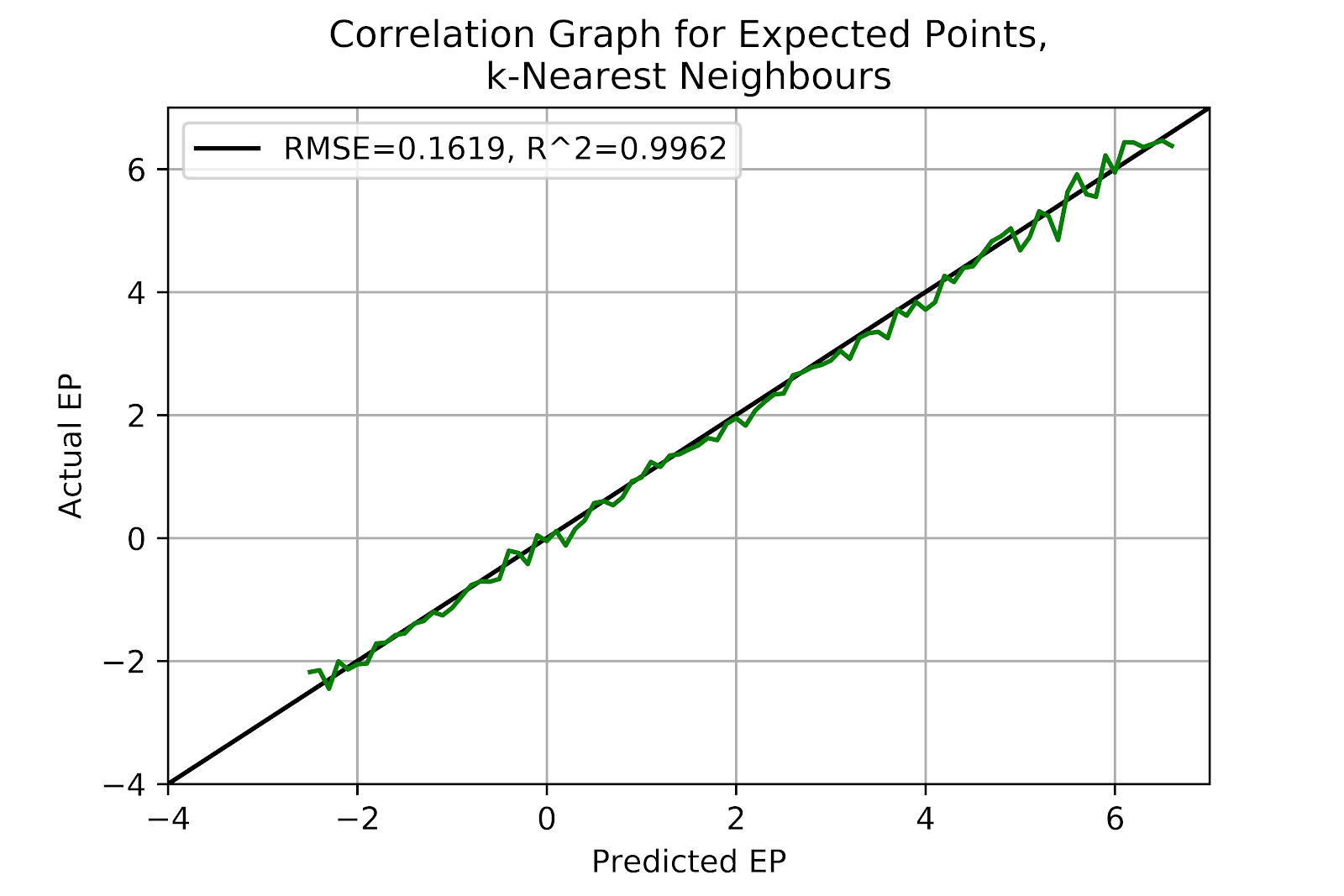
Figure 2 EP Correlation for k-Nearest Neighbours Model

The random forest model shows strong performance in the middle range of EP values, while slightly over-predicting at the high end. Unfortunately, the model massively under-predicts EP at the low end. Figure 3 shows that the under-prediction is so severe that it exceeds the scale of the figure, meant for more reasonably well-calibrated models. This may be situational, related to either specific downs or quarters, which will be further discussed, but this model’s performance pales so far in comparison to the well-calibrated kNN model.

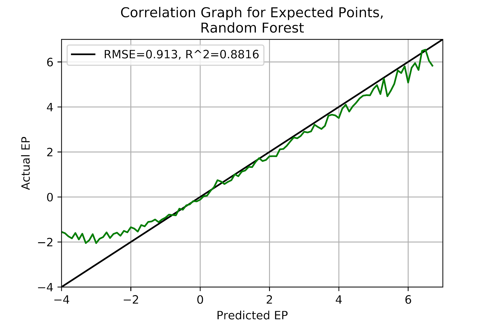
Figure 3 EP Correlation for Random Forest Model

The multi-layer perceptron offers slightly better performance than the k-nearest neighbours model, albeit at the cost of vastly increased computation time. The model is well-calibrated and unbiased across its entire range. Since this model was created with an abundance of hidden nodes, it is unlikely that altering the number of nodes is likely to result in improved performance. In Figure 4 we see the MLP is more stable at higher EP, in comparison the the slight inconsistencies of the kNN model in Figure 4.

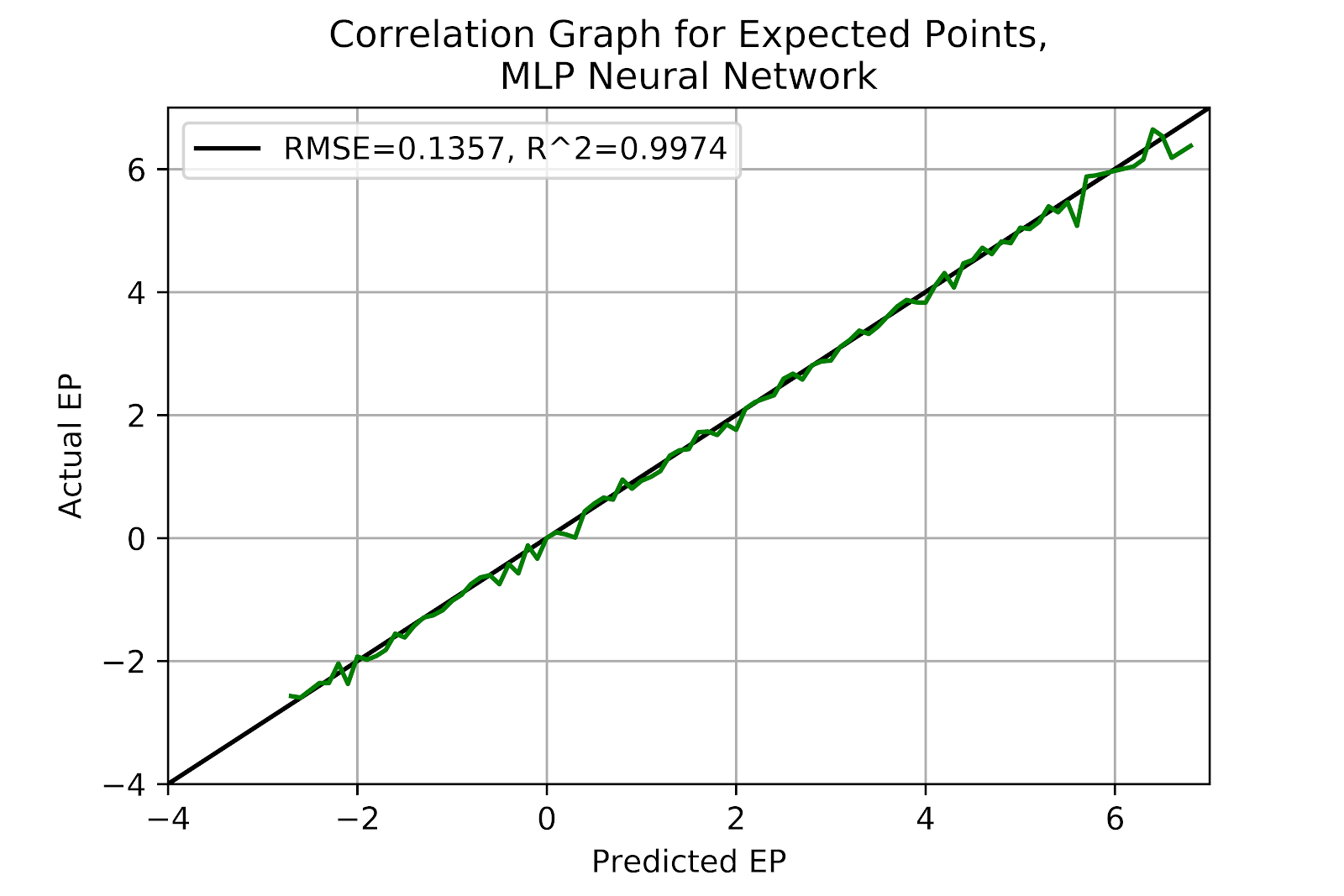
Figure 4 EP Correlation for Multi-Layer Perceptron Model

The Gradient Boosting model shows almost as strong performance as the MLP model, save that it has a slight region of under-prediction at the lower extreme of its range in Figure 5, akin to the random forest but far less severe.

Figure 5 EP Correlation for Gradient Boosting Classifier Model

Of the five models so far, three have shown promise with strong general correlation graphs: k-nearest neighbours, multi-layer perceptron, and gradient boosting. Each model will also have to withstand scrutiny at the down and distance level, as the goal is to find a model that is robust across all situations, but especially in those situations where EP decisions are more common and more critical.

b. By Quarter

EP models are strongest when we can make use Krasker’s infinite first quarter assumption (Krasker 2005). Conversely, they should become less effective as the game goes one, or rather as Win Probability (WP) drifts to the extremes. To retain their universal validity the input features are restricted to down, data, and field position. There has been no filtering of data based on arbitrary definitions of when games become WP. A WP-based metric for filtering data would be a future development, following the development of a well-calibrated WP model. As a proxy, correlation graphs were made for each model on a quarter-by-quarter basis as well as the overall correlation. In each case the resultant data was compared against the idealized function y=x to calculate R2 and RMSE as measures of fit. These are all given in Table 6.

Model	Metric	1st	2nd	3rd	4th
Logistic Regression	RMSE	0.5201	0.4941	0.4904	0.5210
Logistic Regression	R2	0.9597	0.9616	0.9647	0.9467
k-Nearest Neighbours	RMSE	0.2480	0.2090	0.2385	0.3339
k-Nearest Neighbours	R2	0.9899	0.9931	0.9907	0.9769
Random Forest	RMSE	0.4407	0.4237	0.3873	0.6735
Random Forest	R2	0.9670	0.9724	0.9756	0.9074
Multi-Layer Perceptron	RMSE	0.2545	0.2165	0.2246	0.3345
Multi-Layer Perceptron	R2	0.9905	0.9935	0.9927	0.9780
Gradient Boosting	RMSE	0.2344	0.2284	0.2019	0.3875
Gradient Boosting	R2	0.9920	0.9927	0.9940	0.9732

Table 6 Comparison of Correlation Measurements for Different Models by Quarter

The logistic regression model, while not particularly well-calibrated, holds its shape across all four quarters in Figure 6. Consistently under-predicting at the edges and over-predicting in the middle, with greatly diminished performance at higher values. Curiously, we even see a similar peak, between 4.5 and 5 points, where the model strongly underpredicts, before the error decreases, and increases again toward the edge. This pattern is not consistent enough to suspect any particular mechanism behind it, but it is a curiosity worthy of mention. The correlation metrics are stable across the first three quarters, with a slight deterioration in the fourth quarter, as expected when WP concerns overtake EP concerns late in the game.

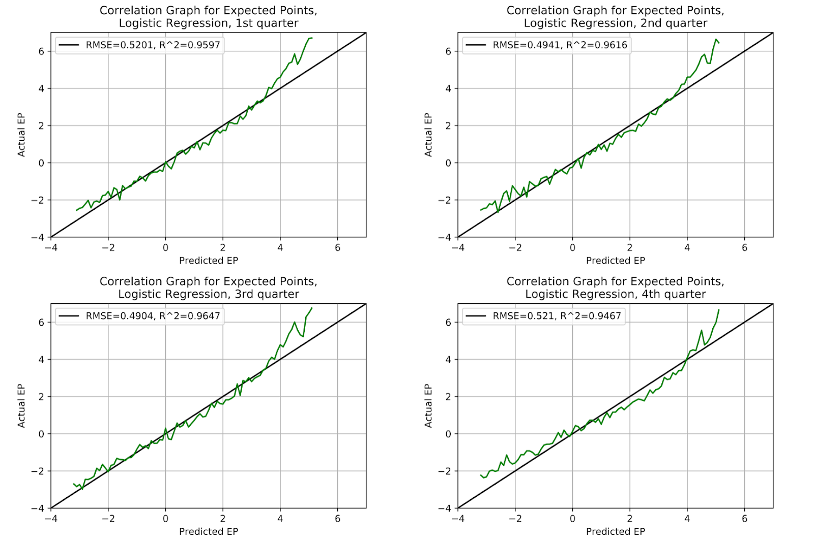
Figure 6 EP Correlation for Logistic Regression Model, By Quarter

Despite the non-standardized data, the kNN model remains model across the first three quarters in Figure 7. Fourth down shows a degree of over-prediction at the upper end and underprediction at the lower end, likely a result of teams with a lead playing conservatively, and teams trailing forced to score. Across all quarters the kNN model is superior to the logit model above in Figure 6, with additional improvements available with future parameter tuning.

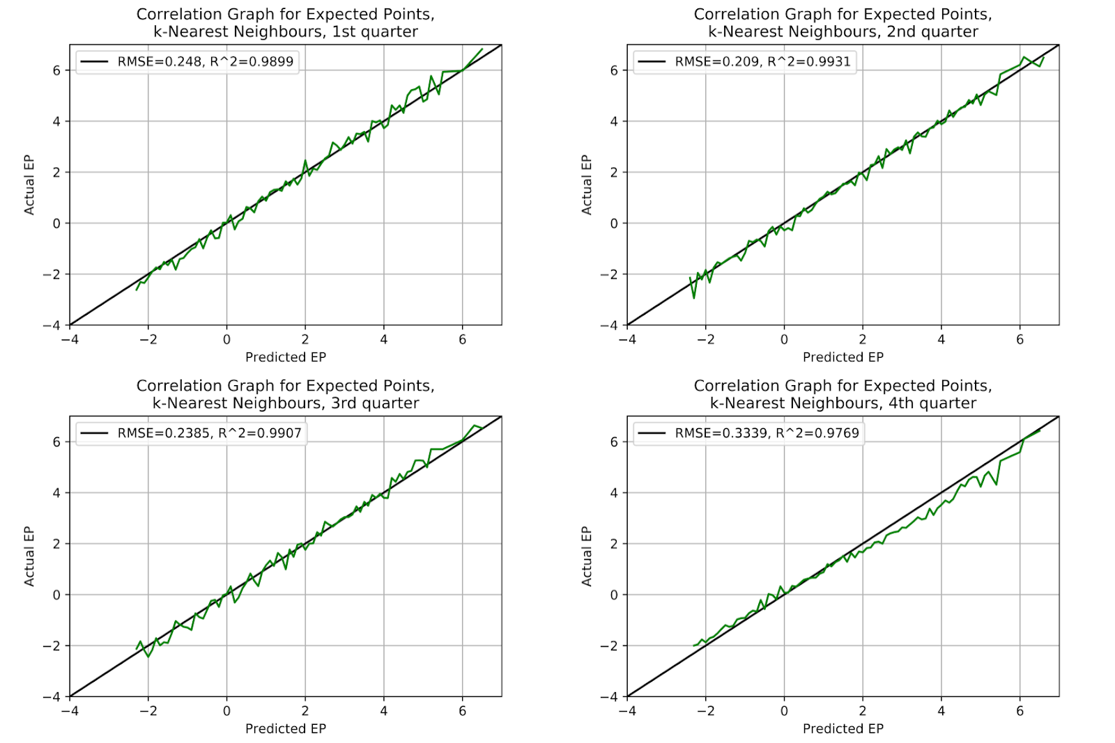
Figure 7 EP Correlation for k-Nearest Neighbours Model, By Quarter

The problems with the random forest model that were seen in Figure 3 persist here in Figure 8 when the model correlation is broken down by quarters. The model is consistently predicting extremely low EP values that are not found elsewhere in other models, and these are consistently shown to be erroneous. The model would frankly be improved if all estimates below -2 EP were simply moved to -2. While this would obviously be a methodological nightmare it fairly illustrates the problems inherent to the model. In the fourth quarter there is also a tendency to over-predict higher EP values, but this is generally a more forgivable offense because it is also seen in other models, and it happens in the fourth quarter, where we would expect discrepancies like this. Table 6 shows that the RF model is almost as poor as the logistic regression model, and in some cases worse. Both these models have consistently poorer correlation metrics than any of the other three.

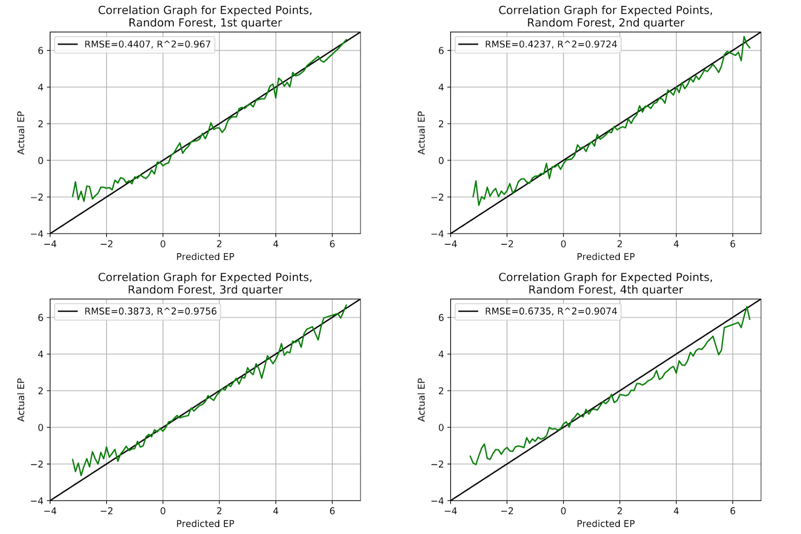
Figure 8 EP Correlation for Random Forest Model, By Quarter

The multi-layer perceptron model in Figure 9 continues to be well-calibrated, and with the exception of some slight bias in the fourth quarter consistent with, but less severe than, what has been previously seen in the k-nearest neighbours model in Figure 7 and random forest model in Figure 8.

Figure 9 EP Correlation for Multi-Layer Perceptron Model, By Quarter

As with the MLP model in Figure 9, the gradient boosting model holds up very well. The same bias is seen in the fourth quarter, and as this has been seen in four of the five models, it can be safely assumed that this is a property of the fourth quarter, and not a product of the models. By extension, Figure 10 shows the logistic regression not expressing this error, which may speak more to the problems inherent in the logistic regression model than with the other models.

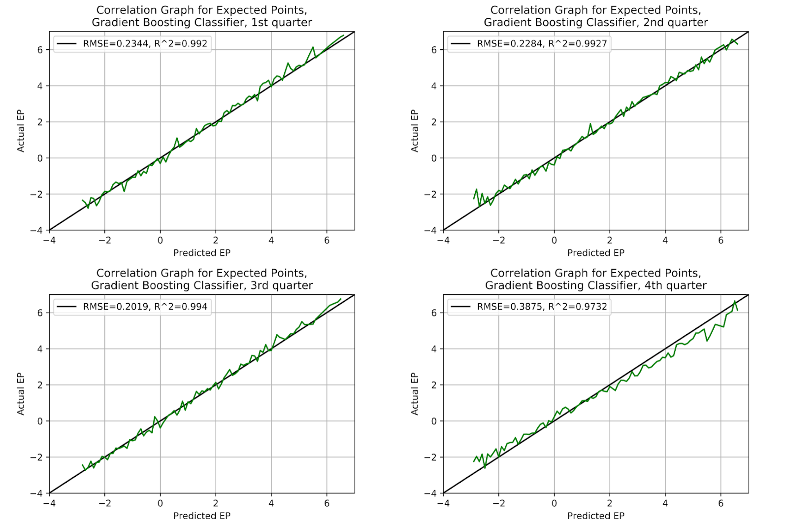
Figure 10 EP Correlation for Gradient Boosting Classifier Model, By Quarter

When looking at the five different models in toto, there is an emergent pattern - each model is fairly consistent in its strengths and weaknesses. The logistic regression model has serious issues and is unlikely to be a candidate for future discussion, and the random forest model has different, but equally serious issues. The other three models, k-nearest neighbours, multi-layer perceptron, and gradient boosting, are all very similar in the measured results and in the visual comparison of their quarter-by-quarter correlation graphs.

c. By Down

To continue the comparison of different models we look at the models in more specific situations. Separating by down is the simplest way to accomplish this task, and removes one of the variables from the system. Table 7 shows the RMSE and R2 of each correlation graph, separated by model and down.

Model	Metric	1st	2nd	3rd
Logistic Regression	RMSE	0.5021	0.5090	0.3997
Logistic Regression	R2	0.9502	0.9471	0.9609
k-Nearest Neighbours	RMSE	0.3118	0.2189	0.7429
k-Nearest Neighbours	R2	0.9838	0.9910	0.8499
Random Forest	RMSE	0.3164	0.6714	0.8550
Random Forest	R2	0.9824	0.9095	0.7884
Multi-Layer Perceptron	RMSE	0.1849	0.1689	0.2064
Multi-Layer Perceptron	R2	0.9941	0.9953	0.9896
Gradient Boosting	RMSE	0.2359	0.2558	0.2174
Gradient Boosting	R2	0.9905	0.9886	0.9879

Table 7 Comparison of Correlation Measurements for Different Models by Quarter

i. 1st Down

The set of plays at 1st & 10 across all points of field position provides a good opportunity to compare apples to apples in a context where the “true” value is not only known, but known to within a reasonable accuracy. Raw EP is can be calculated and confidence intervals then bootstrapped, with 1000 bootstrap iterations to find the 95% confidence intervals. In Table 8 we see the results of fitting a linear regression to the plotted data of 1st & 10 (or 1st & Goal where field position is within 10 yards). This linear regression is plotted using scipy.optimize.curve_fit (Oliphant 2007). As has been seen in all other EP models, EP for 1st & 10 is roughly linearly correlated with field position (Clement 2018b). This is not exactly correct, as EP rises more sharply as the offense approaches the end zone, and flattens when backed up, but it serves as an approximation, at least insofar as the slope is generally representative of the marginal EP value of a yard. Furthermore, it serves as a proxy for congruence between two models.

Model	Slope	Intercept	RMSE	R2
Raw Data	-0.0740	5.855	0.2666	0.9870
Logistic Regression	-0.0698	5.542	0.2634	0.9858
k-Nearest Neighbours	-0.0732	5.794	0.2515	0.9882
Random Forest	-0.0740	5.858	0.2669	0.9870
Multi-Layer Perceptron	-0.0742	5.869	0.2604	0.9877
Gradient Boosting	-0.0740	5.856	0.2608	0.9876

Table 8 Linear Regression Results for EP models, 1st & 10

Looking at Figure 11 we see the raw value of EP on 1st down by field position. Certain individual data point stand out: at the 5-yard line EP is far, far below any of its neighbours. This may be a curious outlier of no significance, but it may also represent the presence of a flawed arbitrary cutoff in playcalling systems. Many teams will employ a specialized short-yardage package for goal line situations, and if teams are using the 5-yard line as a round number cutoff at which to switch their style it may be that this is the wrong point. From the 4-yard line in the data not only rejoins the existing trend, but actually increases in value more steeply than across the rest of the field.

1st & 10 is the most important EP value to determine, as it is the basis for 3rd down decision making, an important topic of future research. When making a 3rd down decision it is important to be forward-looking. The EP value of the 3rd down position itself is not relevant to the decision-making process, only the outcomes of the different options matters, and most of those options result in a 1st & 10 situation.

At the 75-yard line (-35 in common parlance), we see a point where the confidence interval is much smaller than any other point around it, and where the value is lower than expected. As to the smaller confidence interval, this is because there are a disproportionate number of plays that start from this field position, as it is the field position granted to the defense after a field goal, a rouge, or a safety is scored. The larger sample size means that the confidence interval shrinks, as the value of this position becomes more certain. As to why the value is lower, many of the instance where a team starts from exactly the -35, and not merely on or around the -35, they have just given up a field goal. Field goals are, unsurprisingly, scored more often by better teams, and require that an offense at least drive well into opposing territory. The team receiving the ball would then be, on average, worse than their opponent. While some of these drives also come from teams surrendering safeties intentionally, which would tend to have the opposite effect on the EP value of the -35 yard line, this is a less common outcome.

Because of this, it is important to use a model for EP values when preparing 3rd down decisions, because in this case a curiosity of the rules causes approximately 0.5 point difference in the value of the -35 yard line relative to where it “should” be. The point at the -35 yard line is not unique simply because of its distance from the regression line, but because it is the only point more than 10 yards from either end zone whose confidence interval does not include the regression line.

Figure 11 EP Graph for Raw Data, 1st & 10

The logistic regression graph for 1st & 10 EP shows the source of some of the problems with under-prediction for higher EP values. EP values within the 10-yard line for the raw data in Figure 11 are above the fit line, but for the logistic regression model in Figure 12, despite the fit line having a lower intercept and flatter slope, the values are below the fit line.What should be the highest possible EP values are being grossly understated. In the area where EP is at its highest and decisions have the most immediate impact in being translated from expected points to realized points the model is falling well outside the confidence intervals of the raw data.

Figure 12 EP for Logistic Regression Model, 1st Down

The correlation for the logit model on 1st down in Figure 13 is no surprise, the impact of the erroneous goal-line estimations is clearly apparent above 4 EP. The model is concave, almost quadratic in nature, with significant under-prediction at the low end, showing that there is a problem with the model near either goal line, when accurate predictions are most needed.

Figure 13 EP Correlation for Logistic Regression Model, 1st Down

The k-nearest neighbours model shown in Figure 14 is a far better representation of the raw data. Indeed, for certain points such as the -35-yard line there are enough instances of that situation to exceed the number of neighbours considered in the model, and so the model only considers instances from exactly the same situation. Since there are hardly any cases of 1st & 11 or 1st & 19 (1st & Goal notwithstanding), nor for 1st & 12 or 1st & 8, the kNN model for 1st & 10 operates as a smoothing function across field position.

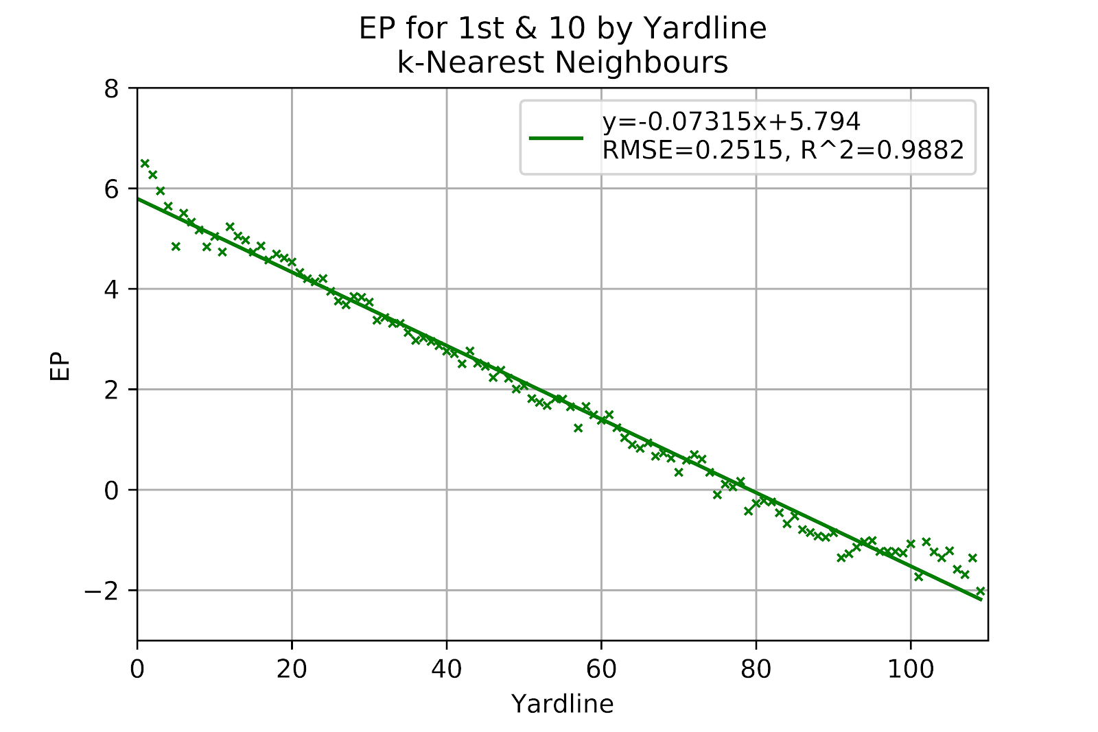
Figure 14 EP for k-Nearest Neighbours Model, 1st Down

At the far left edge of the correlation graph in Figure 15 there is an under-predicted region. This occurs because 1st & 10 plays near ones own goal line are fairly rare, and so they incorporate instance from a greater radius. However, there are no data points beyond the goal line, so to find the requisite number of neighbours the model can only search looking forwards, thereby disproportionately selecting plays with better field position, and thus higher EP.

Figure 15 EP Correlation for k-Nearest Neighbours Model, 1st Down

The performance of the random forest on 1st down in Figure 16 is far better than what has been seen so far. Without distance as a significant factor the model performs much better, and is almost a perfect recreation of the raw data in terms of slope, intercept, RMSE, and R2. All of the unusual points are faithfully recreated, including the discontinuity at the 5-yard line, and the -35-yard line, while the data near either goal line is almost identical to the raw data. Canonically, random forests do not overfit (Breiman 2001), but that may be a more applicable statement to binary classification forests, as opposed to the current multiclass problem

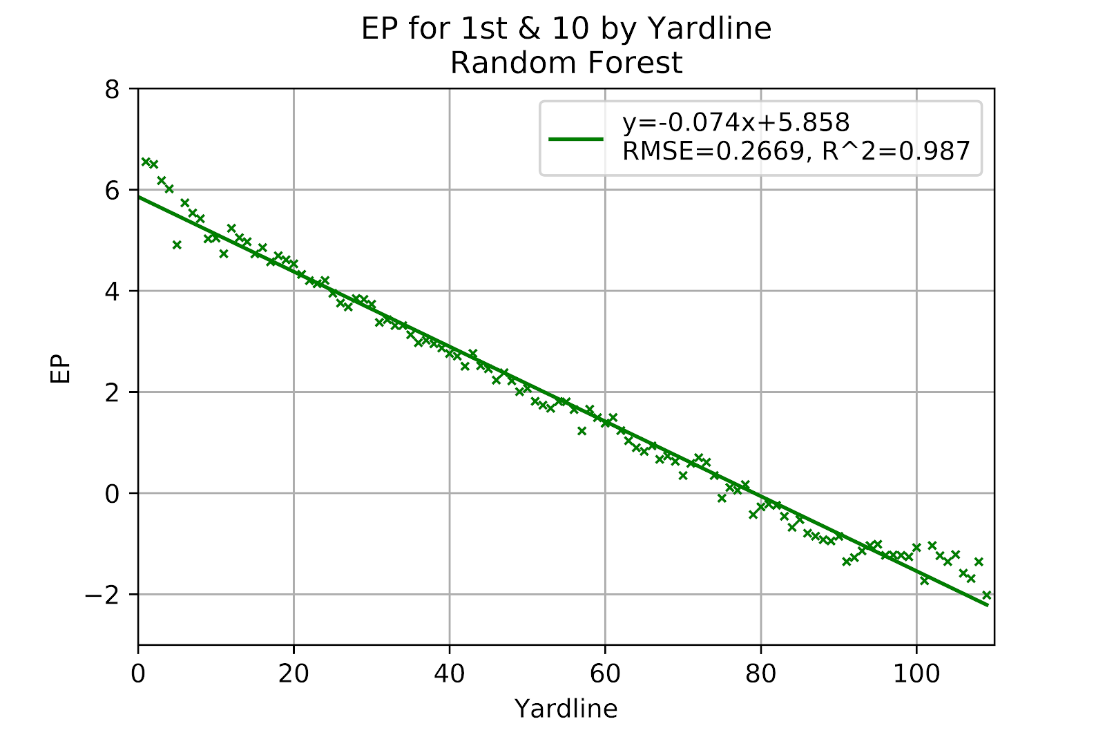Figure 16 EP Correlation for Random Forest Model, 1st Down

In spite of previous poor performance in Figures 3 and 8, the random forest model correlates very well for 1st down, which could have been safely surmised from the similarity in the representations of the EP results of the RF model and the raw data in Figures 16 and 11, respectively. The slightly under-predicted region may have the same root cause as the kNN model, but is small enough that it may simply be a product of randomness.

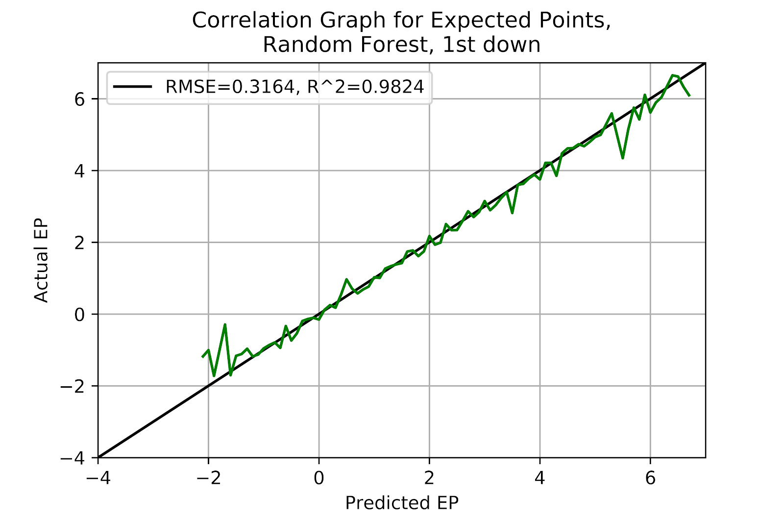
Figure 17 EP for Random Forest Model, 1st Down

The MLP model in Figure 18 is also a very good fit, hewing very close to our raw data. At a glance it is difficult to see any distinction between the MP and RF models, and the raw data. This becomes a recurring theme in all the models save the logit mode, whose issues have previously been discussed.

Figure 18 EP for Multi-Layer Perceptron Model, 1st Down

The regression line for the random forest model is a more exact replication of the raw data, but the MLP model has a much better correlation, and without the localized issue at the left edge of the correlation graph in Figure 19 the MLP model inspires greater faith in its validity, especially when considering the overall better performance seen in the general correlation graph and the quarterly correlations.

Figure 19 EP Correlation for Multi-Layer Perceptron Model, 1st Down

The GBC model, shown in Figure 20 is also a very close representation of the raw data. If we consider the game of footballoon a theoretical level, any improvement in field position is a good thing, and should result in increased field position. Therefore a plot of EP for 1st & 10 such as we have in Figure 11 for some idealized perfect model should show a monotonically decreasing function. However, our models are designed around the minimization of errors based on the raw data, and when the data space is well-populated the model will fit the data given more than any theoretical understanding of the game. An advantage to the logit function is that this holds true, EP is monotonic with respect to both distance and field position.

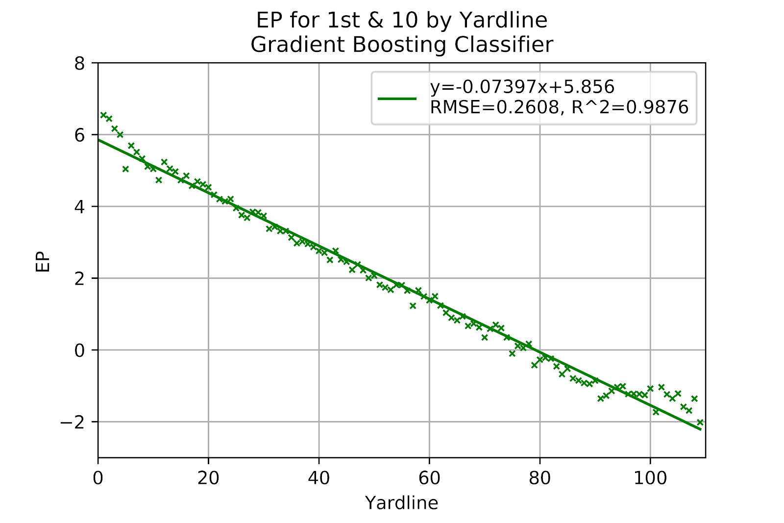
Figure 20 EP for Gradient Boosting Classifier Model, 1st Down

The GBC model is well-correlated in Figure 21, close behind the MLP model. As with the random forest there is a small area at the lower end of the graph where the model underpredicts, but this is only four data points, and it seems equally likely that this is noise rather than signal.

Figure 21 EP Correlation for Gradient Boosting Classifier Model, 1st Down

Because of the large quantity of data for each point in the raw data, most models are able to replicate this faithfully, which is a desired feature when the data is already sufficient to have good confidence without necessarily a need to add a model. EP for 1st & 10 is already able to be calculated to good precision by simply using the raw data, and so this may be the least important down to use a model, but the value of the model on 1st down is two-fold. First, to consider situations of 1st down where the distance to gain is not 10 yards, and second, to have a consistent methodology to apply when determining EPA of individual plays.

ii. 2nd Down

Since the overwhelming majority of 1st down plays are 1st & 10, we can look at them in isolation, ignoring the small portion of 1st down plays that are not 10 yards (or & goal). For other downs this does not hold. 2nd down exists over a range of distances, which we here have set a cutoff at 25, beyond which there are few plays, and very few of them at any specific distance. The interplay of distance and field position demands that we look at the picture in toto, rather than, say, separating the data into individual graphs by distance or plotting separate curves for each distance. Heatmaps allow the representation of three-dimensional data in a two-dimensional image, and while they do not offer the kind of that a scatter plot might, they are better at conveying the general sense of trends across both axes, especially with noisy data. The legend at the right is consistent across all models, with red at the upper end of scoring, and blue at the lower end, following a rainbow pattern between the two.

Figure 22 shows the raw data of EP for 2nd down. Note that there are two blank triangles in the heatmap, one at the upper left and another at the lower right. These are the impossible combinations of down & distance, where either the distance to gain is greater than the field position or the line to gain would be shy of the -10-yard line. Other blanks appear in the raw data because there are combinations of distance and field position that have not occured in the dataset.

It comes as no surprise that EP is largely a produce of field position, as the heatmap fairly continuously changes colour along the lower axis. There is also a general sense of decreasing EP with increasing distance, but this is a much noisier tendency, especially as data is sparse at longer distances.

Figure 22 EP for Raw Data Model, 2nd Down

In Figure 23 we see the heatmap for logistic regression on 2nd down, and it is here that the limitations of logistic regression come through. Since logistic regression produces a set of continuous function the heatmap is entirely continuous. While this is certainly plausible as a first assumption we see that there is a strong central tendency bias from this model. In the lower left corner we see none of the rich reds that we see in Figure 22, and in the upper right none of the dark blues and purples. The model is timid, and understates the extremes of EP, compressing all values into a narrow range.

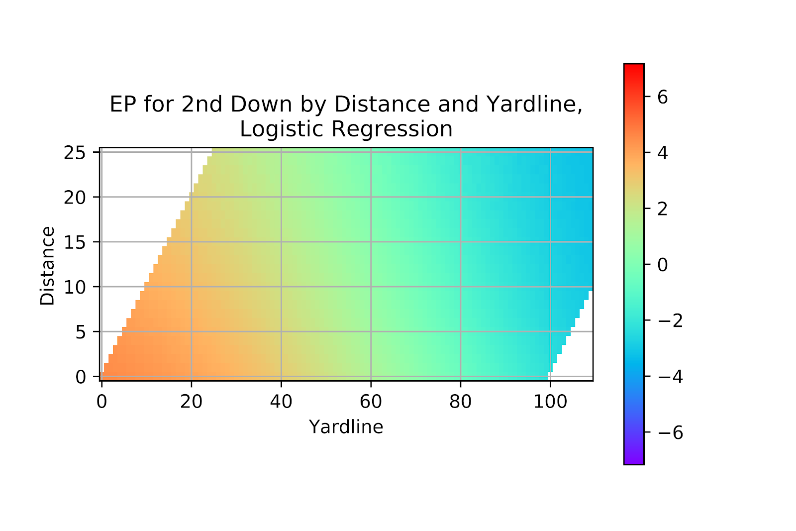
Figure 23 EP Correlation for Logistic Regression Model, 2nd Down

The correlation graph for logistic regression on 2nd down in Figure 24 supports the visual evidence from Figure 23 as with all the other examinations of the logit model in Figures 1, 6, and 13 the model is consistently too timid. There is massive underestimation at the higher EP values, and again at the lower values, balanced by general overestimation in the middle. A model that is consistently in error by a fixed amount is workable, as most EP calculations are concerned with the relative differences in EP values, but this model swings between different errors, and to extreme degree near the goal line.

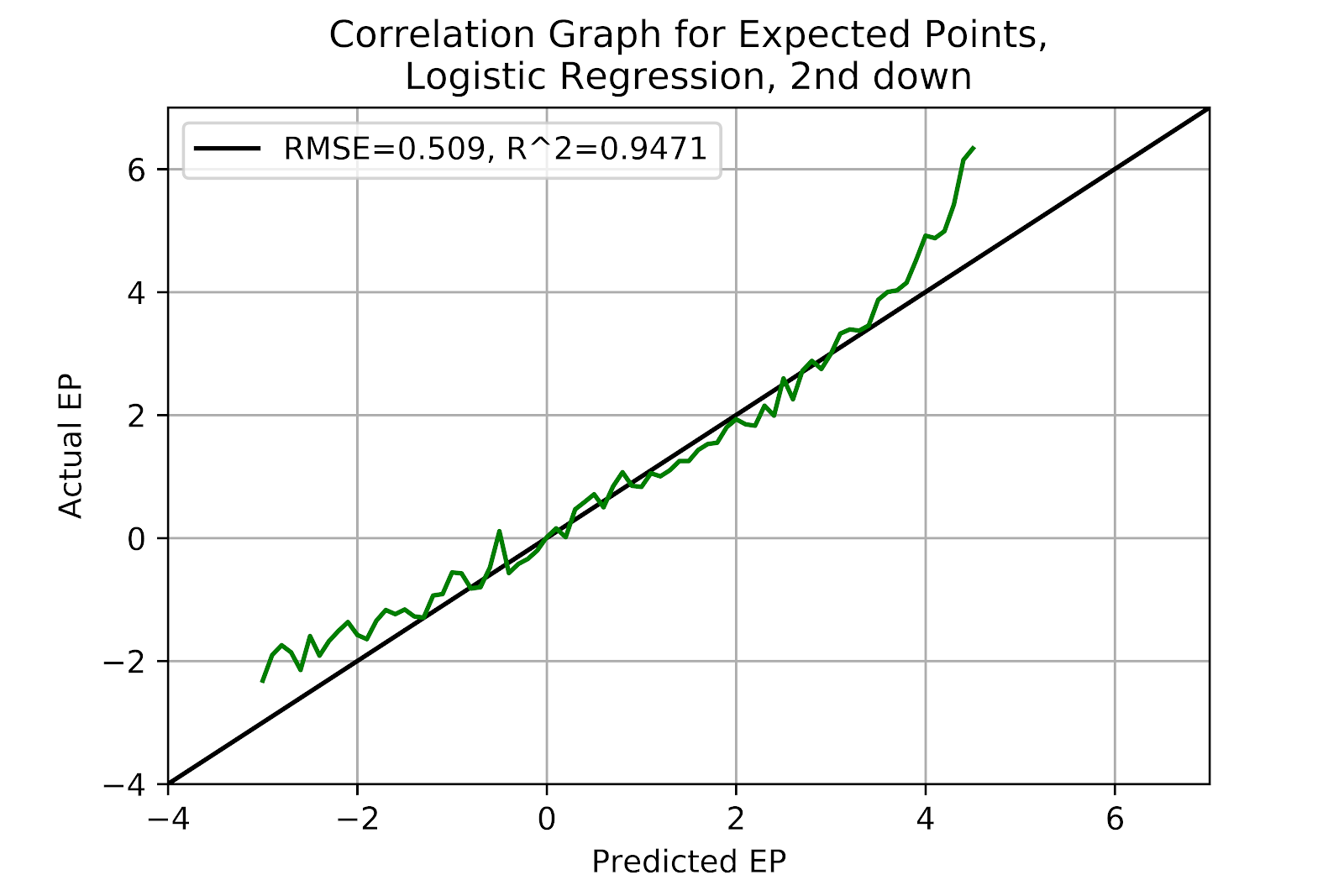
Figure 24 EP for Logistic Regression Model, 2nd Down

The k-nearest neighbours model in Figure 25 is better than the logistic regression one in that it does properly show the higher EP values in the lower left. But it still does not show the values in the upper right as being as strongly negative as we can clearly see in the raw data of Figure 22. We can surmise that this is because of the limited data at the extremes of distance and field position the model is forced to reach more and more into more favourable offensive positions and begins averaging data that is not truly representative. This could be rectified in one of two ways: First, a scaling factor could be used to penalize data taken too far away from the point of interest, but this would require significant tuning to optimize and the attendant risk of overfit. Alternately, a radius neighbours classifier could be used, but this would absolutely require standardization of the data and tuning the radius, both of which could be prone to overfit. Furthermore, the large difference in data density between different parts of the space, as well as certain spaces being more sensitive to small changes than others would make the radius a very difficult parameter to tune.

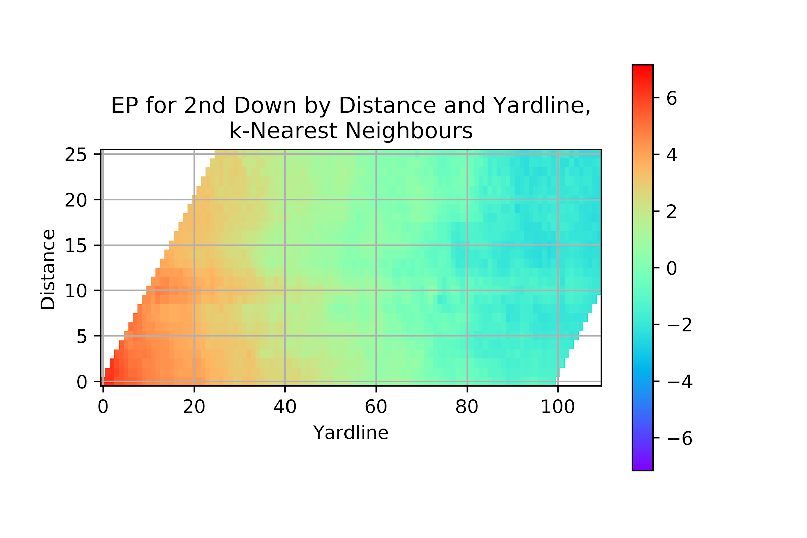
Figure 25 EP for k-Nearest Neighbours Model, 2nd Down

The kNN model is as well-calibrated for 2nd down as it has generally been for all situations. Figure 26 has good metrics, and no sign of systemic error. We might recall from Figure 15 that on 1st down the kNN model had trouble at the extremes because the data is bounded by the goal lines, forcing an asymmetric selection of neighbours. This does not present itself here on 2nd down. While it certainly occurs, these situations appear rare enough not to have made an impact on the correlation graph.

Figure 26 EP Correlation for k-Nearest Neighbours Model, 2nd Down

The random forest output for 2nd down in Figure 27 bears the strongest visual resemblance to the raw data of Figure 22. This is not a compliment. Unsurprisingly, the raw data contains a lot of cases where an unexpected result occurred from a very specific scenario that sits alone in its data bin. Despite efforts to combat this, the RF model shows signs of overfitting the data, even when cross-validating. Although the model could be tuned by adjusting tree depth and leaf size this goes away from the very core philosophy of random forests, and would make this random forest model more akin to a convoluted k-nearest neighbours model.

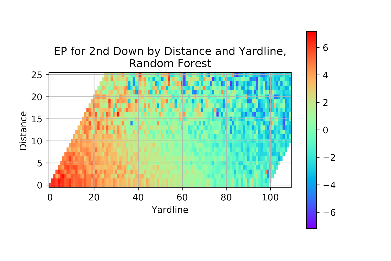
Figure 27 EP for Random Forest Model, 2nd Down

The correlation graph in Figure 28 for the random forest model on 2nd down is an utter abomination. The lower end of the graph continues to be a complete mess as the model insists on predicting very low EP values that are simply not supported by the reality on the field, and compensates for this by predicting high EP values that are similarly not supported by reality. The R2 is atrocious and the model simply has no business being used in any applied context.

Figure 28 EP Correlation for Random Forest Model, 2nd Down

The MLP model in Figure 29 shows a continuous shift in colours, and does properly show higher values of EP where we would expect them. It does not show the extremely low EP values, but this then raises the question of whether those values are correct; should we be seeing EP values of less than -4 points? Even if a team faces 2nd & 25 on their own 1-yard line, is it reasonable to assume that their opponent is nearly guaranteed to score a touchdown? This model appears to bottom out around -3 points, around the same place as the logistic regression, and slightly lower than the k-nearest neighbours model. It is about where the raw model values 1st & 10 at the 1 yard line. We can assume then that this model is somewhat understating how bad some of the extreme positions are, but without a more complete dataset at the fringes of distance to gain it becomes difficult to truly set a floor for EP. The ceiling of EP is always equal to the value of a touchdown, and while the theoretical flow is simply the negative value of a touchdown, in practical terms this is not reachable or even approachable, the simple act of punting will force the opponent to successfully advance the ball to score, to say nothing of the possibility of successfully converting the distance.

Returning to the lower part of the heatmap, where the majority of the game is played, we do notice a slower transition from the reds to the greens than in the raw model. This appears to be the effect of field goal range. While kickers are not identical, they are fairly similar, and the conversion rate for a field goal increases quickly with field position once the kick is at all feasible. This model shows a much more gradual transition, though not so much as our logistic regression model.

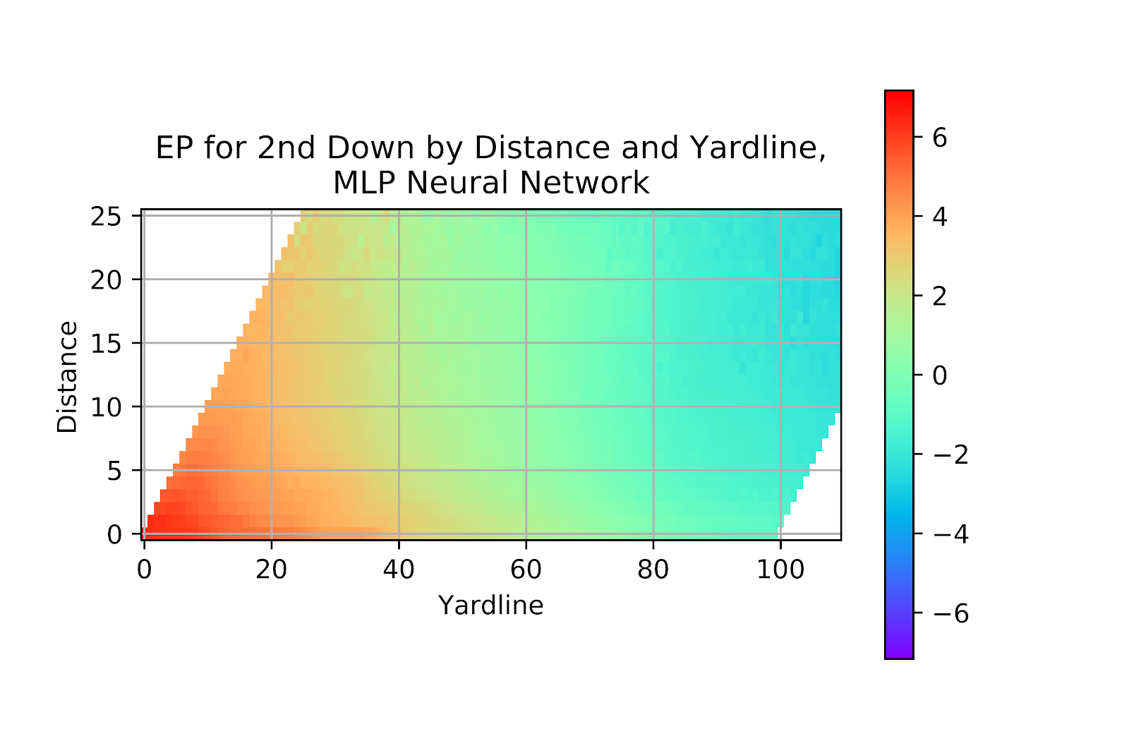
Figure 29 EP for Multi-Layer Perceptron Model, 2nd Down

As with every angle from which our results have been viewed, the multi-layer perceptron holds up in the correlation in Figure 30 as well as it does in the heatmap. Again showing the strongest correlation metrics of all the models, The MLP model is currently the model to beat.

Figure 30 EP Correlation for Multi-Layer Perceptron Model, 2nd Down

The gradient boosting model in Figure 31 looks like a rougher version of the MLP model. We see important features including a broad dynamic range, even broader than the MLP as it includes some deeper blues in the upper right corner, and the presence of the field goal range line. Some slight discontinuities at extreme ranges are acceptable, given the relative rarity of these cases.

Figure 31 EP for Gradient Boosting Classifier Model, 2nd Down

The correlation graph of the GBC model in Figure 32 betrays the apparent benefit of the increased range of the model in Figure 22, showing that the GBC model has a tendency to underpredict very low EP values. While certainly not as problematic as seen on the random forest model the GBC model proves generally less well-calibrated than the MLP or kNN models for 2nd down.

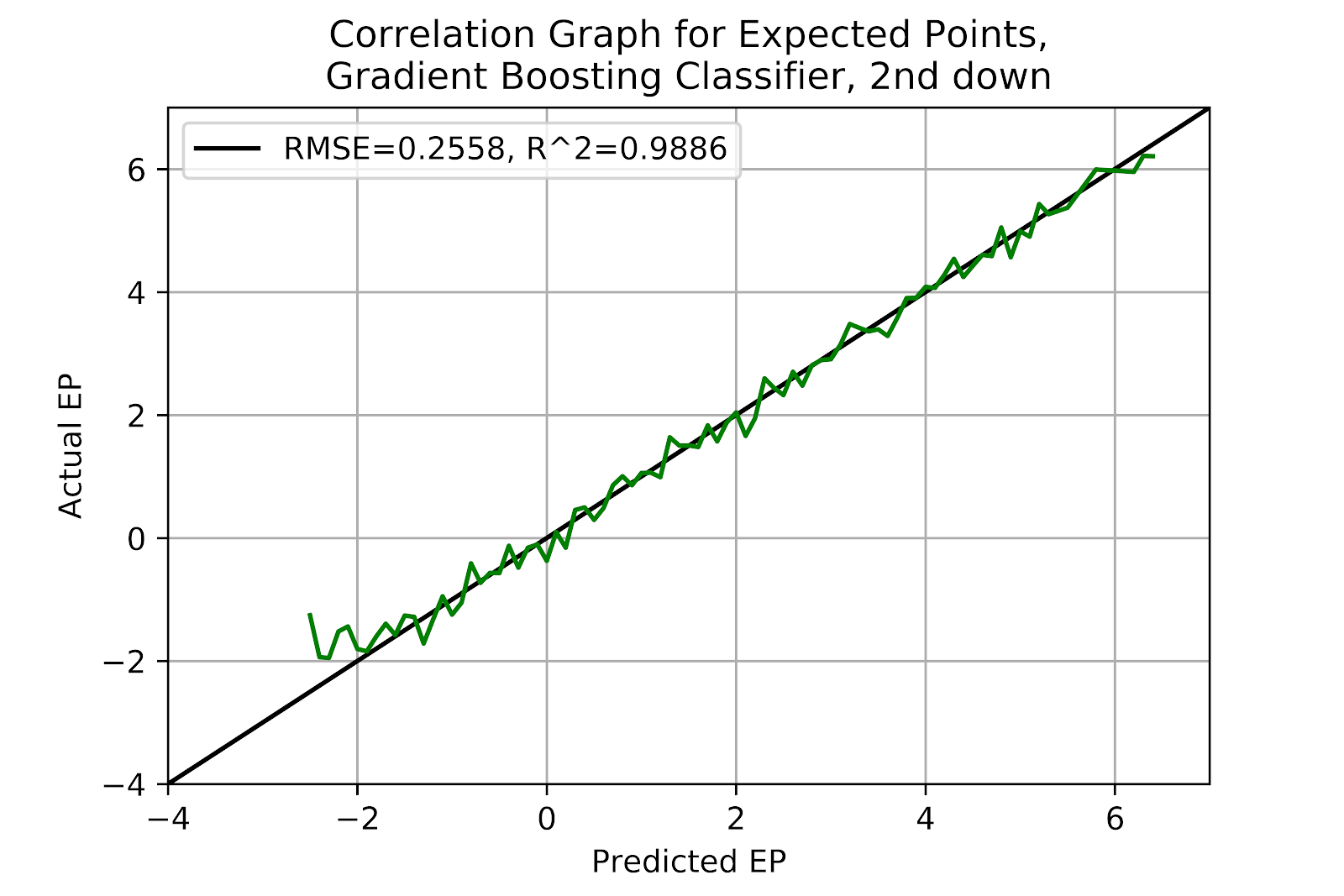
Figure 32 EP Correlation for Gradient Boosting Classifier Model, 2nd Down

While the multi-layer perceptron model continues to impress, the k-nearest neighbours model is perhaps the most impressive model when one considers the simplicity of the model and the lack of any parameter tuning.. The gradient boosting model performs well, but not as well as one would hope given the computational intensity of the model, while the random forest disappoints and the logistic regression model raises concerns about many extant models currently in use.

iii. 3rd Down

The assessment of 3rd down EP is difficult, as the value of a 3rd down is dependent on the choice the offense makes. The offense has, nominally, four basic options. They can attempt to convert the distance, they can kick a field goal, they can punt, or they can concede an intentional safety. But by calculating the average value of a 3rd down situation we can calculate the expected points added (EPA) of a play, and use this as a measure of play success, as well as for future work.

Figure 33 shows the raw data for 3rd down. 3rd down has the least data, and therefore the noisiest heatmap. It also has lower EP values overall, with the total range of values being compressed, limiting the ability to distinguish the values of adjacent blocks. We can see field goal range clearly delineated, as well as the value for 3rd & 1 being much higher than 3rd & 2, irrespective of field position, as has been noted in previous work on P(1D) (Clement 2018d).

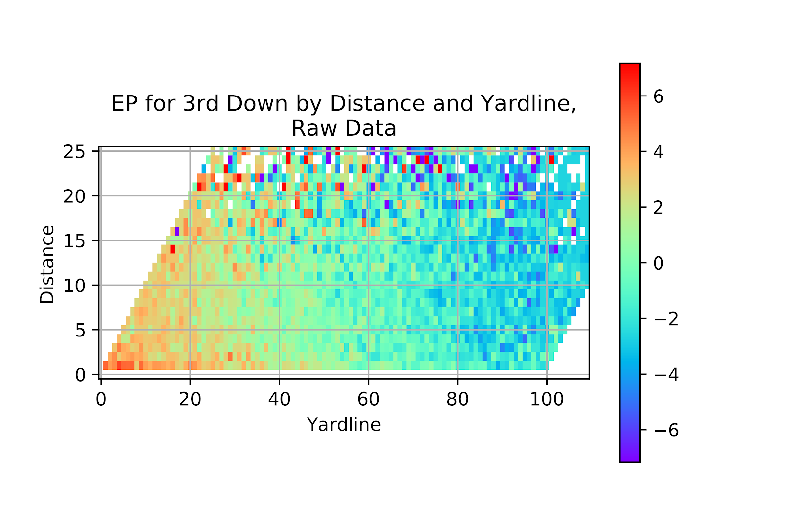
Figure 33 EP for Raw Data, 3rd Down

The logit model for 3rd down in Figure 34 is essentially a transposition of the 2nd down version, as logit models are wont to do. There is insufficient dynamic range in the values and not enough discontinuity at 3rd & 1 to trust this model as more than a first approximation. Furthermore, where we would expect to see field goal range represented as a near-vertical band of colour, since EP(FG) is unrelated to distance to gain, this does not occur.

Figure 34 EP for Logistic Regression Model, 3rd Down

The correlation graph in Figure 35 strikes the death knell for the logit model. It continues to perform terribly, with underestimation rampant at both ends of the EP spectrum and overprediction in the middle. Interaction terms may provide an improvement in performance for this model, but it seems improbable that it would bring the model’s performance in line with that of its competitors.

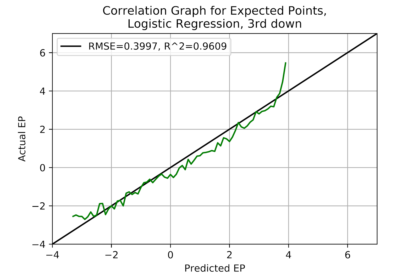
Figure 35 EP Correlation for Logistic Regression Model, 3rd Down

With k-nearest neighbours we get a far better picture than with logit. A richer set of reds near the goal line is seen in the lower-left corner of Figure 36. Field goal range is better represented, and we see EP values push deeper into the negative numbers. While for 2nd down it is normal for distance to have a strong effect on EP because of its impact on P(1D), on 3rd down there are relatively few conversion attempts, and for the other three options (field goal, punt, and safety) the distance to gain is irrelevant. So it is unsurprising that we should not see a strong effect along the vertical axis once we are more than a few yards from the line to gain.

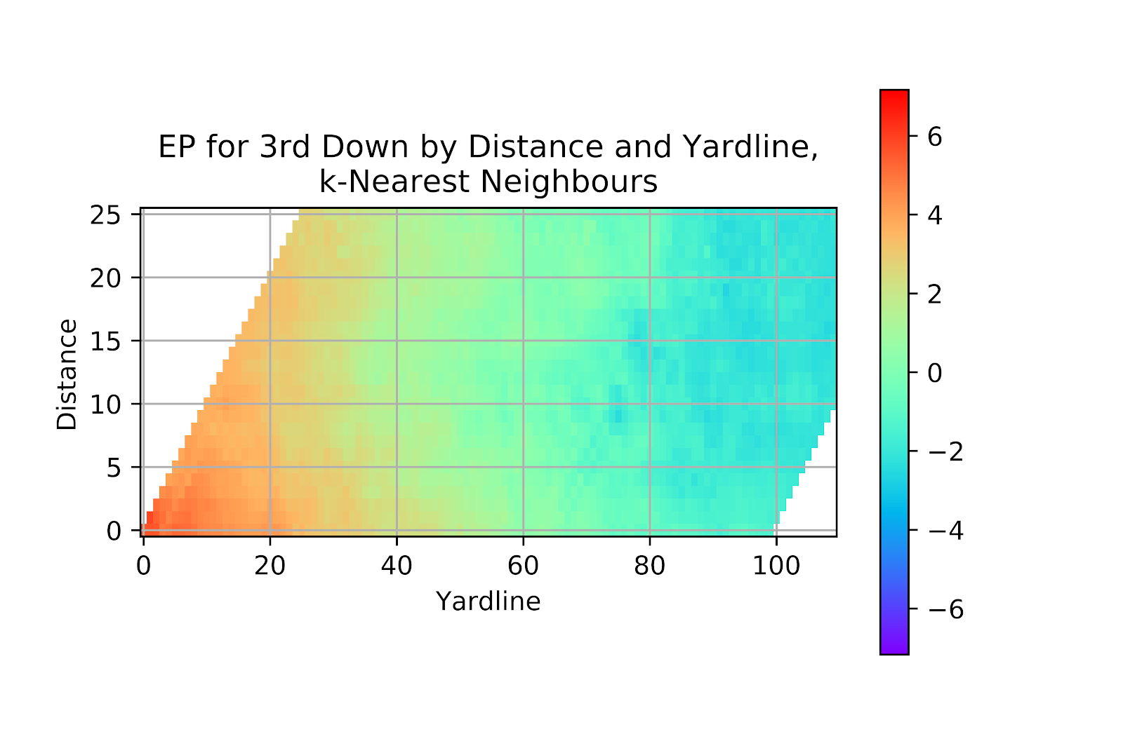
Figure 36 EP for k-Nearest Neighbours Model, 3rd Down

Despite k-nearest neighbours modelling being a pleasant surprise so far, the correlation graph in Figure 37 brings a swift end to this positivity. The model manages to overpredict across the board, and by no small margin. We see the worst correlation metrics of any correlation graph so far, and we can only conclude that there is some hidden effect, or that some error exists elsewhere. In short, the kNN model is utterly unusable for 3rd down EP estimates.

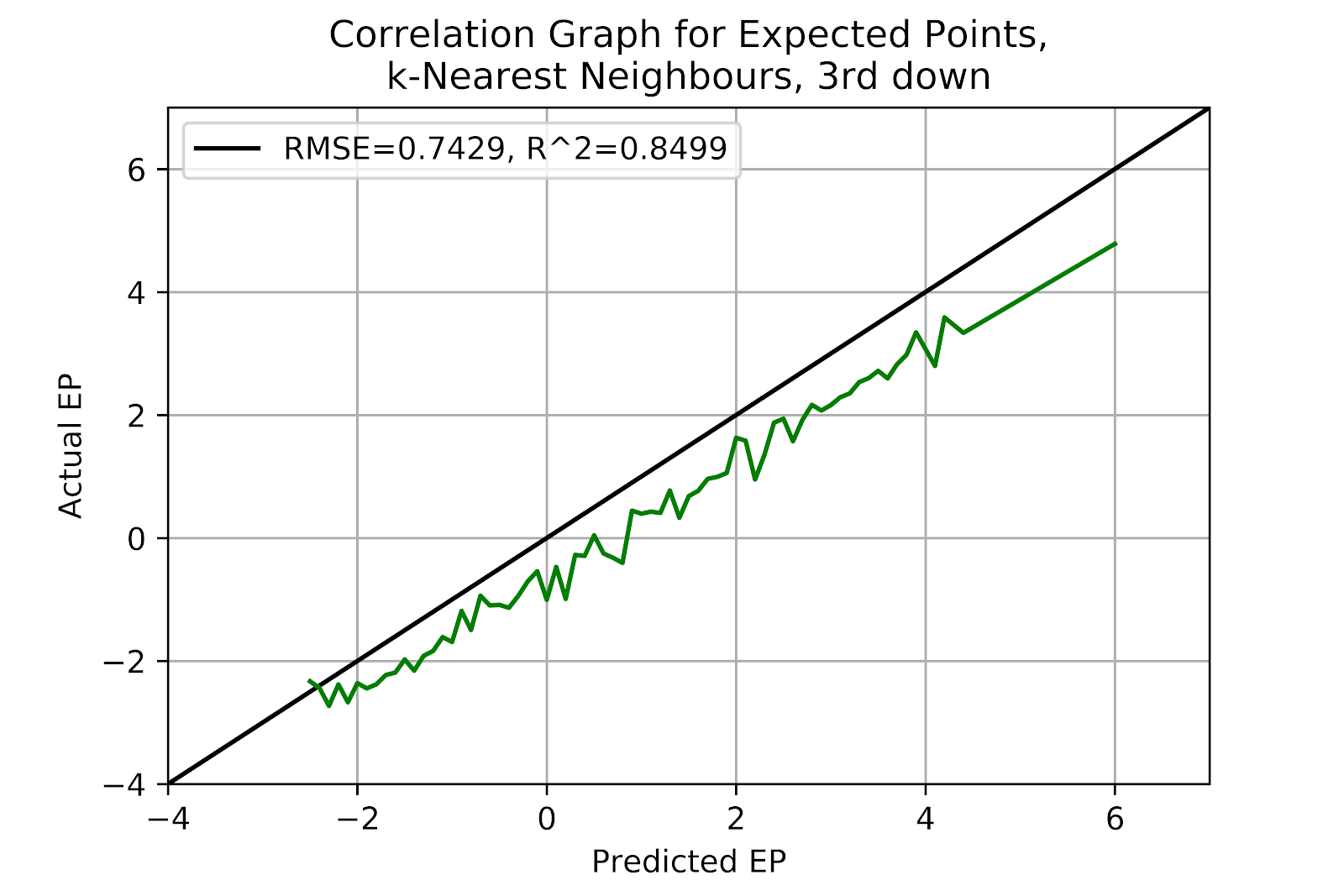
Figure 37 EP Correlation for k-Nearest Neighbours Model, 3rd Down

The problems for the random forest model continue in Figure 38, where the output too closely resembles the raw data, and we see a great deal of discontinuity in the more sparsely populated regions of the heatmap, with high EP values coming from areas that do not make sense.

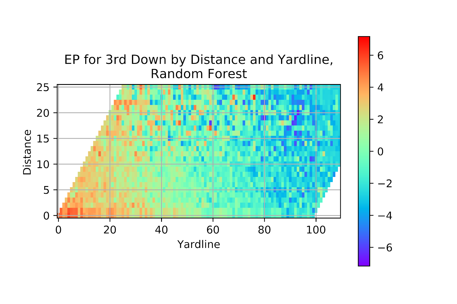
Figure 38 EP for Random Forest Model, 3rd Down

And the correlation graph in Figure 39 shows that the random forest does not benefit from 3rd down more than any of the other scenarios. The random forest cannot help itself from predicting extremely low EP values, and yet it also overpredicts at the other end.

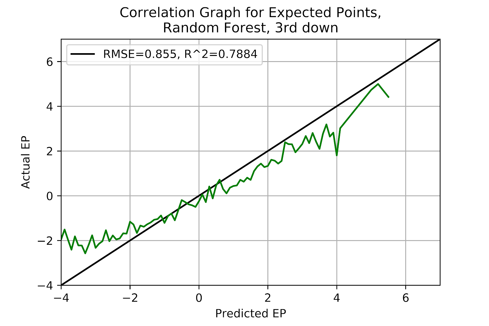
Figure 39 EP Correlation for Random Forest Model, 3rd Down

The MLP model in Figure 40 is consistent with our expectations of 3rd down EP. EP increases as both distance and field position decrease, and 3rd & 1 is considerably more valuable than 3rd & 2. The EP values for distance <10 are consistent with what we see in the raw data, giving us confidence that longer distances are well-estimated as well.

Figure 40 EP for Multi-Layer Perceptron Model, 3rd Down

The MLP model remains well-calibrated in 3rd down, remaining the best model in yet another situation. As 3rd down has the sparsest data there is a degree of roughness in the correlation graph in Figure 41.

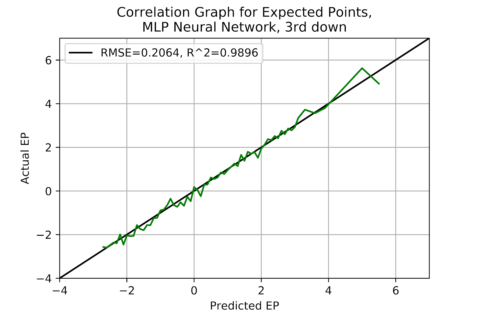
Figure 41 EP Correlation for Multi-Layer Perceptron Model, 3rd Down

The gradient boosting model shown in Figure 42 provides an interesting comparison to the previous four models. It shows a greater dynamic range than the logistic regression and k-nearest neighbour models, has continuously decreasing EP across field position, with fairly constant EP over distance, and shows the impact of 3rd & 1. Notably 3rd & 1 is shown as having far greater EP than 3rd & 2, which should be expected because teams often will attempt and successfully convert 3rd & 1, but far less often 3rd & 2, so it would often lead to a punt instead of a continuation of the drive.

Figure 42 EP Correlation for Gradient Boosting Classifier Model, 3rd Down

The GBC model is also well-calibrated in Figure 43, roughly equal to the MLP model. While the GBC model has some areas where lower EP is predicted this does not appear to cause an area of underprediction in the correlation, unless one considers a very small region that could well be a random artefact.

Figure 43 EP for Gradient Boosting Classifier Model, 3rd Down

The results of each model on 3rd down only serve to confirm prior suspicions about the relative strengths of the models. While the smaller dataset on 3rd down means that all models suffer, models that performed well on 2nd down perform well on 3rd down, and the ways in which models succeed and fail do not change.

5. Conclusion

Having developed five models of EP and comparing them in different ways we are able to draw some conclusions about the utility of models. Despite the popularity of logistic regression models for EP in other football leagues (Yurko, Ventura, and Horowitz 2018; Clement 2018b), the work here shows that, at the very least, this model is not appropriate for U Sports football. It is conceivable that the addition of an interaction term between distance and field position would improve the model’s quality, it seems unlikely that it would supplant some of the other models seen here. It raises questions about all of the logistic regression EP models seen elsewhere, and how those plots correlate

The random forest model also proved a major disappointment, performing almost as poorly as the logistic regression model. Its strong 1st down performance belied the serious problems on 2nd and 3rd down. Conversely, the k-nearest neighbours model proved a very pleasant surprise, one that could be even more interesting with proper parameter tuning. While the GBC model performed admirably, it was ultimately the MLP model that was the most consistent performer across all scenarios.

Unexpectedly, none of the models showed massively reduced 4th quarter performance relative to the other three quarters. While model performance generally declined in the 4th quarter It appears that play is not hugely altered in the 4th quarter. While play styles obviously change in the end-game, this shift does not seem to set in until later in the 4th quarter.

As far as the actual value of EP is concerned, we are not met with any great surprises. EP peaks with 1st & Goal at the 1-yard line, and is inversely correlated with both yardline and distance to gain. Indeed the determination of exact EP values for specific combinations of down, distance, and field position is far less interesting than the general trends and the ability to effectively model these values, since the relative difference between two plays is the more important measure.

Having a sound and verifiable EP model opens the possibility of a 3rd down decision calculator based on EP, the examination of kicking plays based on EP, and is a preliminary step in the development of a WP model. It also allows the determination of EPA for individual plays and therefore the comparison of different play features based on EP. Expected Points is the most versatile and widely-used metric in football analytics, and bringing it to U Sports will help to bring the league forward into a new, data-driven world.