1-Abstract
P(1D) values across down and distance were calculated for CFL data across down & distance. & Goal situations were separated and viewed independently. Results were compared to results obtained using the same methods on U Sports data. CFL offenses generally follow the same trends as seen in U Sports in terms of P(1D), though CFL P(1D) is consistently ~5 percentage points higher than U Sports under the same conditions. 1st down follows the same linear trend, while 2nd down shows exponential decay, with the previously discussed “Stupidity Asymptote” at 10%. However, CFL teams are markedly less willing to attempt 3rd down conversions, causing a lack of usable data points for 3rd down. For & goal situations the disparity between CFL and U Sports P(1D) does not seem to be as prevalent.
2-Introduction
Having already determined P(1D) values for U Sports football (Clement 2018b), and subsequently developed a database of CFL play-by-play data (Clement 2018c), the reuse of the methods to determine P(1D) in U Sports football made it possible to quantitatively look at P(1D) in the CFL, and to directly compare the two leagues.
Following best practices for replication, the code and methodology from the previous work were followed as exactly as possible. That is, certain labels were changed, especially for trivial matters such as sheets being named “CIS” or “CFL,” or other details not relevant to the results. In the parser every possible effort was made to ensure that, despite the differences in the layout of the data, the output would be consistent and correct.
3-P(1D)
This data set has a total N=189, 760, of which we consider all offensive plays from scrimmage with distance to gain <=25, a total of 139, 949 plays. In the analysis we only consider points with N>100. While the 25-yard cutoff is consistent with the prior work, in practice there are no situations where distance is greater than 22 and N>100. The distribution of data by down & distance is given in Table 1.
Distance
|
1st Down
|
2nd Down
|
3rd Down
|
1
|
11
|
3712
|
2303
|
2
|
2
|
3155
|
357
|
3
|
2
|
3462
|
223
|
4
|
3
|
3836
|
175
|
5
|
622
|
4674
|
175
|
6
|
2
|
4091
|
125
|
7
|
2
|
3952
|
87
|
8
|
5
|
3343
|
68
|
9
|
6
|
2632
|
64
|
10
|
76513
|
14544
|
378
|
11
|
7
|
1707
|
40
|
12
|
15
|
1234
|
94
|
13
|
28
|
842
|
65
|
14
|
15
|
650
|
56
|
15
|
1246
|
1186
|
50
|
16
|
11
|
449
|
25
|
17
|
10
|
416
|
27
|
18
|
17
|
381
|
19
|
19
|
13
|
304
|
16
|
20
|
1216
|
664
|
14
|
21
|
1
|
139
|
7
|
22
|
106
|
8
| |
23
|
1
|
96
|
5
|
24
|
63
|
4
| |
25
|
75
|
98
|
5
|
Table 1 Distribution of Data by Down & Distance
Similar to U Sports data, data for 1st down is clustered at multiples of 5 yards, the result of penalties. 1st & 10 is far and away the most populous data point, for obvious reasons, monopolizing 54.6% of all the plays. 2nd & 10 is the second most-populated bin, the result of incomplete passes and runs for no gain on 1st & 10. Otherwise, 2nd down has a fairly equal distribution for all distances less than 10, declining thereafter. Thus far everything concurs with the distribution of U Sports data. 3rd down, however, is rather different. The CFL data has a similar number of plays at 3rd & 1 (2792 vs 2303), despite the disparity in the size of the overall data sets. Thereafter the CFL data shows far fewer 3rd down attempts proportional to the amount of data. CFL teams are seem to attempt far fewer third downs of distances greater than 1.
To explain this split between two ostensibly parallel data sets, we might posit a few hypotheses: First, it may be that CFL teams are more likely to convert second downs, irrespective of distance, giving them fewer opportunities to attempt third downs. In this case we would expect a higher P(1D) for 2nd down, and a similar P(1D) for 3rd down. To some extent this is difficult to measure because there are fewer data points at 3rd down that reach the N=100 threshold.
Alternately, it may be that CFL games have greater parity. U Sports games being more often an unbalanced competition there is more often one team being forced into progressively more desperate 3rd down attempts. A third possibility is that U Sports kicking games are far less effective than CFL teams, and so there are more situations where going for it on 3rd down is the best option, and also that coaches in both teams are cognizant of this and adjust their planning accordingly. It is certainly reasonable to assume the U Sports kickers are, on average, less talented than their professional counterparts, and that the disparity between them is enough to alter the calculus of third-down decisions.
Finally, it may well be that CFL coaches are far more inclined to punt out of concerns for job security. Regardless of the rationality of attempting third down conversion in various situations, public perception places blame on coaches for failed attempts, and so coaches receive perverse incentives to punt, in an example of risk aversion over odds. Job security in the CFL being more tenuous than in U Sports, coaches are incentivized to deflect the perception of fault.
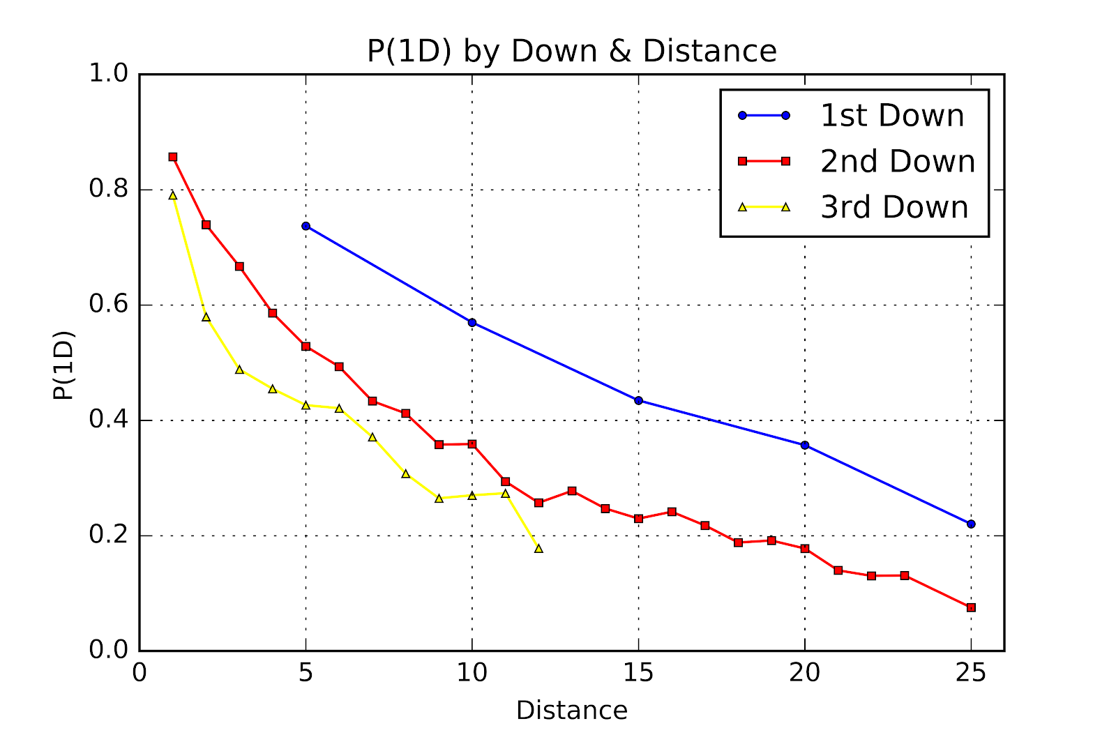
In Figure 1 we see an overall picture of P(1D), with all three downs plotted together. The general trends of each down seem to generally follow those of the U Sports data. P(1D) decreases with increasing distance, as expected, and P(1D) decreases with increasing down as well. Again we see a more linear trend on 1st down, and a convex shape on 2nd down. Unfortunately the scarcity of data points on third down frustrates our efforts to find a general trend. 
Figure 1 P(1D) by Down & Distance
A table showing the numerical values of the points shown in Figure 1 is included in Table 2. At a glance we see that P(1D) of 1st & 10 in the CFL is quite a bit higher than in U Sports, (0.6188 vs 0.5698), a sign of offenses being better at advancing the ball. P(1D) at 2nd & 10 is also 5 percentage points higher in the CFL (0.4044 vs. 0.3589), showing stronger passing offenses relative to defenses. In recent years changes to CFL rules have caused more of a divergence from the amateur rule book, creating more penalties to the offense’s benefit on passing plays, perhaps explaining some small part of the difference. In fact we see an across-the board difference of roughly 5 percentage points for the CFL over U Sports. That this is done with remarkably fewer 3rd down attempts makes the unwillingness to go for it even more remarkable. p-values comparing the two leagues were calculated for all qualifying points via the Fisher method, but proved vanishingly small, all less than 10-5 and most too small to be calculated.
Distance
|
1st Down
|
2nd Down
|
3rd Down
|
1
|
0.8947
|
0.8432
| |
2
|
0.7670
|
0.5938
| |
3
|
0.6794
|
0.4574
| |
4
|
0.6142
|
0.3543
| |
5
|
0.7814
|
0.5804
|
0.4343
|
6
|
0.5182
|
0.4880
| |
7
|
0.4947
|
0.2989
| |
8
|
0.4379
|
0.3088
| |
9
|
0.3982
|
0.4375
| |
10
|
0.6188
|
0.4044
|
0.3624
|
11
|
0.3076
| ||
12
|
0.2990
| ||
13
|
0.3076
| ||
14
|
0.3154
| ||
15
|
0.4856
|
0.2690
| |
16
|
0.2294
| ||
17
|
0.2163
| ||
18
|
0.2336
| ||
19
|
0.2138
| ||
20
|
0.3840
|
0.1913
| |
21
|
0.1439
| ||
22
|
0.1321
| ||
23
| |||
24
| |||
25
|
Table 2 P(1D) by Down & Distance
a-1st Down
Consistent with what was found in U Sports (Clement 2018b) as well as in American football (Clement 2018a), P(1D) for 1st down follows a linear trend, shown in Figure 2, with 95% confidence intervals shown. We see a regression function of y = -0.0266 x + 0.9014with an R2 of 0.9894. The RMSE of 0.0153, and RMSE/µ 0.0230 also point to a good fit. Granted, with only 4 data points it is not unexpected that the correlation coefficients would be strong, though there is no theoretical basis for P(1D) being linearly correlated to distance, and this regression is more illustrative of a trend and of use for interpolation.

Figure 2 P(1D), 1st Down, with Error Bars and Regression Line
The y-intercept at 0.9014 is lower than one would expect from a theoretical approach, where we should see the y-intercept at exactly 1. We see a slope that is 10% steeper than in U Sports, perhaps an artefact of a limited set of points. Still, we are able to see the impact of penalties, such that a 5-yard penalty is worth an average 12.45 percentage points of P(1D). In Table 3 we see the raw data of the points and their confidence intervals, where we see the tight intervals, lending some credence to the notion of extrapolating using the regression line.
Distance
|
Lower CL
|
P(1D)
|
Upper CL
|
5
|
0.7468
|
0.7814
|
0.8132
|
10
|
0.6154
|
0.6188
|
0.6223
|
15
|
0.4575
|
0.4856
|
0.5137
|
20
|
0.3566
|
0.3840
|
0.4120
|
Table 3 P(1D) for 1st Down with 95% Confidence Intervals
b-2nd Down
Data for 2nd down with 95% CIs, plotted in Figure 3, shows the same exponential decay fit as in U Sports, here with the form y = 0.8490 * e-0.1136 * x + 0.1004 across 22 data points. The raw data is given in Table 4.
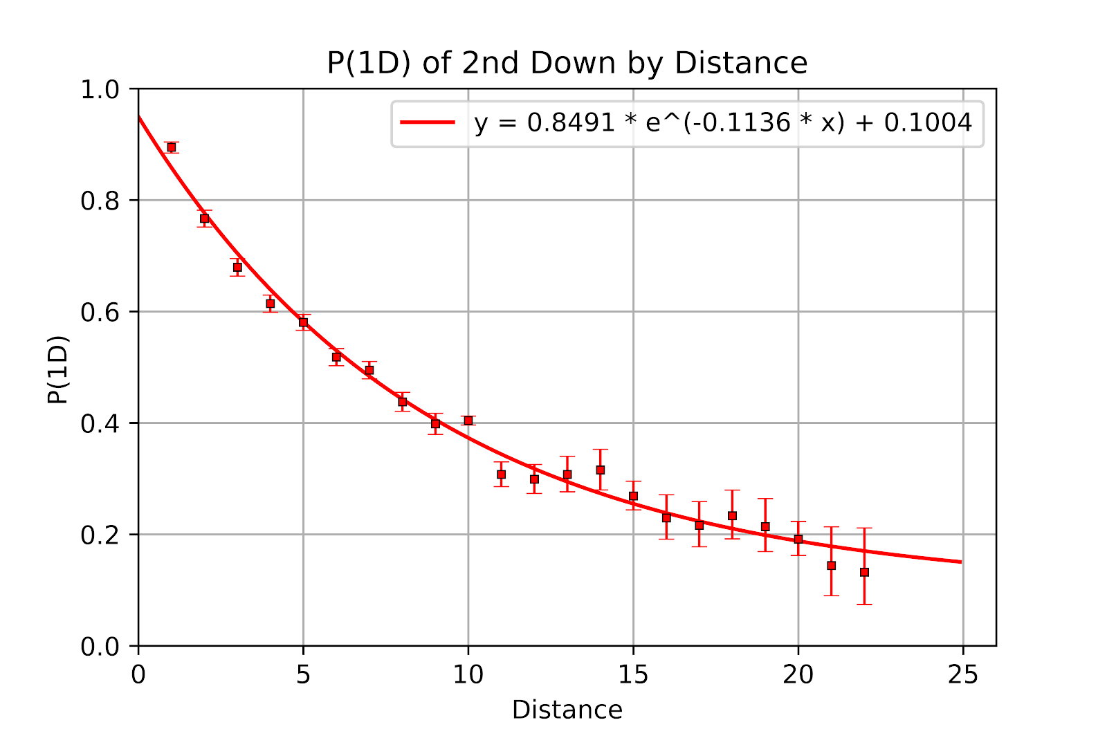
Figure 3 P(1D), 2nd Down, with Error Bars and Regression Line
For measuring the fit we have the pseudo-R2 of 0.9876, RMSE of 0.0227 and RMSE/µ of 0.0578. We see three instances where the fitted curve does not pass through the confidence interval, at 2nd & 1, 2nd & 10, and 2nd & 14. The first two have been previously discussed; 2nd & 1 is much shorter than 1 yard, as it includes every distance of less than 1.5 yards, and 2nd & 10 is populated by teams who threw incomplete passes on 1st & 10, whereas the neighbouring points are more commonly the result of failed runs, and failed runs are more strongly associated with bad teams, while incomplete passes happen to all teams, especially as poor teams will skew more towards the run on 1st & 10. 2nd & 14 may well be the result of randomness, as we would expect to see in a sampling of this size.
As was seen in U Sports we retain the notion of the “Stupidity Asymptote.” The Stupidity Asymptote for U Sports is at 8.34%, but in the CFL our estimate of the Stupidity Asymptote is 10.04%, again likely due to rules and officiating in favour of the offense and a general increase in passing. Unfortunately this dataset ends at 22 yards, there not being enough data at longer distances to include them. The data is included in tabular form in Table 4.
Distance
|
Lower CL
|
P(1D)
|
Upper CL
|
1
|
0.8843
|
0.8947
|
0.9044
|
2
|
0.7519
|
0.7670
|
0.7817
|
3
|
0.6635
|
0.6794
|
0.6949
|
4
|
0.5986
|
0.6142
|
0.6296
|
5
|
0.5661
|
0.5804
|
0.5946
|
6
|
0.5028
|
0.5182
|
0.5336
|
7
|
0.4790
|
0.4947
|
0.5104
|
8
|
0.4210
|
0.4379
|
0.4549
|
9
|
0.3794
|
0.3982
|
0.4172
|
10
|
0.3964
|
0.4044
|
0.4125
|
11
|
0.2857
|
0.3076
|
0.3301
|
12
|
0.2736
|
0.2990
|
0.3254
|
13
|
0.2766
|
0.3076
|
0.3400
|
14
|
0.2798
|
0.3154
|
0.3527
|
15
|
0.2439
|
0.2690
|
0.2952
|
16
|
0.1913
|
0.2294
|
0.2711
|
17
|
0.1777
|
0.2163
|
0.2591
|
18
|
0.1920
|
0.2336
|
0.2794
|
19
|
0.1691
|
0.2138
|
0.2642
|
20
|
0.1620
|
0.1913
|
0.2233
|
21
|
0.0902
|
0.1439
|
0.2134
|
22
|
0.0741
|
0.1321
|
0.2117
|
Table 4 P(1D) for 2nd Down with 95% Confidence Intervals
While the Stupidity Asymptote being as high as 10% is of interest on one level, we can certainly see that the graph of P(1D) is zero-bounded, in that it cannot be negative, and given that with infinite data we would always have the occasional, if exceptionally rare, successful play on 2nd & extremely long, the function must be asymptotic, even if that asymptote is 0. The two most common classes of functions producing horizontal asymptotes are rational functions and exponential decay functions. An exponential decay seems a better choice here, it is found commonly in nature in similar situations, it requires far fewer parameters, and it is more reasonable to argue the the decay rate is continuous with respect to increasing distance than to suggest that a complex construction of polynomials is behind the decline of P(1D) over distance.
c-3rd Down
As has been noted, 3rd down attempts in the CFL are comparatively rare, and largely the province of teams without other options. Figure 4 is therefore limited to only seven data points. While ordinarily this would not justify a regression it has been included here for comparison’s sake, in order to keep continuity with the equivalent U Sports chart.

Figure 4 P(1D), 3rd Down, with Error Bars and Regression Line
While the regression function has been included for the comparison’s sake, it is clear that the data is insufficient to make a meaningful model. With only 7 data points and confidence intervals 15 percentage points wide the function can generously be called “junk.” Our R2 is only 0.9150, RMSE is 0.0458, and RMSE/µ is 0.0908. To argue that the Stupidity Asymptote of 3rd down is higher than for 2nd down is odd and highly unlikely at best, and to suggest that it occurs at over 40% defies all reason. Ultimately we lack adequate data to speak intelligently on the nature of P(1D) on 3rd down in the Canadian Football League. In Table 5 the confidence intervals are shown numerically. In it we see that 3rd & 1 is well-defined with a confidence interval 3 percentage points wide, and fits our general trend across all downs of CFL P(1D) of being 5 percentage points higher than in U Sports, but the regression curve does not even pass through this confidence interval. All other points show too much uncertainty to speak intelligently.
Distance
|
Lower CL
|
P(1D)
|
Upper CL
|
1
|
0.8277
|
0.8432
|
0.8579
|
2
|
0.5409
|
0.5938
|
0.6452
|
3
|
0.3907
|
0.4574
|
0.5252
|
4
|
0.2836
|
0.3543
|
0.4300
|
5
|
0.3597
|
0.4343
|
0.5112
|
6
|
0.3976
|
0.4880
|
0.5790
|
10
|
0.3139
|
0.3624
|
0.4131
|
Table 5 P(1D) for 3rd Down with 95% Confidence Intervals
d-& Goal
The value of separating & Goal can be demonstrated by the P(1D) value of 1st & 10 vs 1st & Goal from the 10. Table 6 shows the numerical values of the data graphed in Figure 5. Note that there are no points of distance greater than 10 that qualified for inclusion. The axes of the chart have been left as in all other figures for the ease of comparison, as has the colour scheme of 1st down being blue, 2nd down red, and 3rd down yellow.
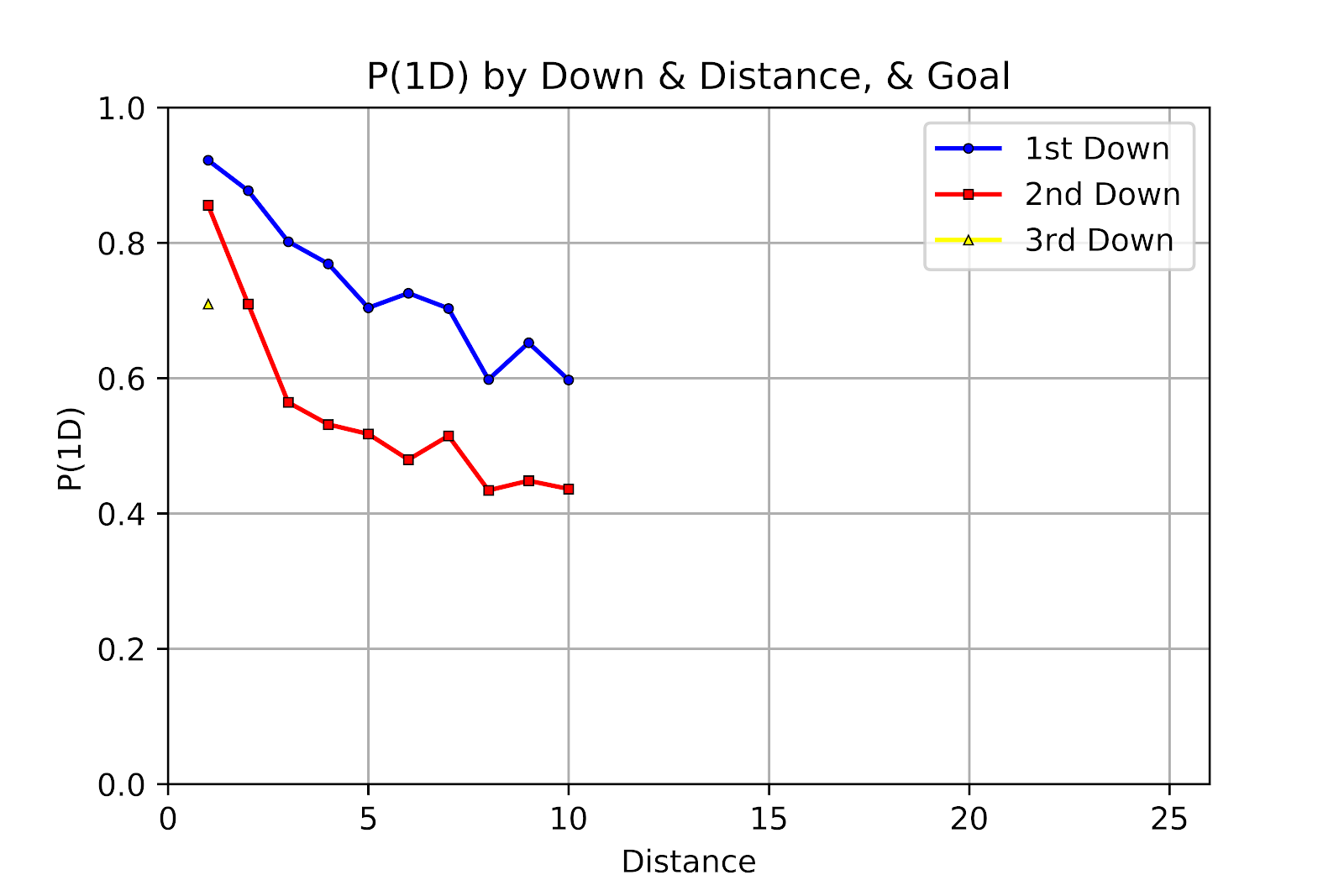
Figure 5 P(1D) by Down & Distance for & Goal
While we see a jump at 2nd & 7 similar to what we saw at 2nd & 7 in U Sports, the confidence intervals of the points overlap too much to confidently state that this is not just a quirk of statistics. The 95% CI for 2nd & 6 ranges from 0.4027 to 0.5571, while that of 2nd & 7 goes from 0.4275 to 0.6012, with a Fisher score of 0.5669. For the present moment, pending the addition of new data from future seasons, we will set this aside.
Whereas all the previous comparisons showed that CFL offenses had a distinct edge over U Sports ones, & goal situations appear to break from that pattern. While acknowledging the greater variance in these results due to the smaller sample sizes, we see that the U Sports results are roughly equal to their CFL counterparts, occasionally even surpassing them, especially on 2nd & short. We have no hypothesis at this time to suggest why this might be happening.
Distance
|
1st Down
|
2nd Down
|
3rd Down
|
1
|
0.9221
|
0.8555
|
0.7097
|
2
|
0.8770
|
0.7097
| |
3
|
0.8018
|
0.5641
| |
4
|
0.7690
|
0.5316
| |
5
|
0.7039
|
0.5174
| |
6
|
0.7256
|
0.4795
| |
7
|
0.7031
|
0.5147
| |
8
|
0.5979
|
0.4341
| |
9
|
0.6522
|
0.4483
| |
10
|
0.5974
|
0.4362
|
Table 6 P(1D) by Down & Distance for & Goal
While CFL teams’ aversion to 3rd down attempts has previously been discussed, Table 7 shows N values for down & distance combinations of & Goal situations. With the exception of 3rd & 1 there is an absence of 3rd & Goal attempts. A future examination of EP and 3rd down decision-making will be able to confirm suspicions that this decision is oft contraindicated.
Distance
|
1st Down
|
2nd Down
|
3rd Down
|
1
|
757
|
443
|
155
|
2
|
309
|
186
|
30
|
3
|
333
|
195
|
22
|
4
|
355
|
190
|
8
|
5
|
439
|
230
|
18
|
6
|
317
|
171
|
15
|
7
|
320
|
136
|
9
|
8
|
373
|
129
|
4
|
9
|
322
|
116
|
1
|
10
|
467
|
149
|
10
|
Table 7 N Values for & Goal Situations
4-Conclusion
Having provided a complete comparison of P(1D) between the CFL and U Sports, it seems well-established that CFL offenses are more able to advance the ball in a consistent manner and to gain first downs. Perhaps most puzzling here is that while CFL teams consistently show themselves more adept at gaining first downs across all situations, they consistently avoid the opportunity to attempt a third down conversion. To further investigate this phenomenon will require an in-depth analysis of kicking effects as well as EP in both leagues
For future applied research, especially as pertain to the idea of decision-making on 3rd down, it seems that the current data is inadequate to give a reasonable sense of precision, and our regression techniques used above also seem inadequate. The best option, then, may be to use a more sophisticated statistical technique. We might suggest the use of logistic regression here, allowing for a smoother function that naturally incorporates data outside the current bin in a weighted fashion. The primary concern then would be at 3rd & 1. The observation that & 1 situations outperform expectations from the exponential regression and the going theory that it relates to compression and rounding effects means that a logistic regression might not be appropriate here. Instead, it may be best to use the raw calculation of 3rd & 1 or 2nd & 1 and then to use the logistic model for greater distances, or to use alternately the raw data or the regression, whichever has the lesser uncertainty.
5-References
Clement, Christopher M. 2018a. “Keep the Drive Alive: First Down Probability in American Football.” June 3, 2018. https://passesandpatterns.blogspot.com/2018/06/keep-drive-alive-first-down-probability_67.html.
———. 2018b. “Three Downs Away: P(1D) In U Sports Football.” Passes and Patterns. August 23, 2018. http://passesandpatterns.blogspot.com/2018/08/three-downs-away-p1d-in-u-sports.html.
———. 2018c. “Going Pro: Developing a CFL Play-by-Play Database.” Passes and Patterns. August 30, 2018. https://passesandpatterns.blogspot.com/2018/08/going-pro-developing-cfl-play-by-play.html.


No comments:
Post a Comment