1 – Abstract

A continuation of prior efforts to consolidate the body of knowledge in American football analytics (Clement 2018), this work discusses the development of Expected Points as an analytical model over the past decades, with a focus on results, statistical methods, data management techniques, and historiographical change.

The development of EP over the past forty years has shown development in statistical techniques employed, growing from linear approximations based on two data points to advanced smoothing techniques and non-linear fits. This growth is aided by the exponential growth in dataset sizes that has paralleled the rise in cheaply available computing.

2 – Introduction

Expected Points is the evolution of football models after P(1D). It is the most applicable of the families of models, allowing for real-time decision-making in game situations with high confidence over most of a game’s duration. EP strikes a balance between P(1D)’s generalized model and the WP’s specific one. It seeks to assign a point value to a given game state based on an averaging of historical data of future scoring from each state. EP is not appropriate for end-of-half decisions or in desperate comeback situations, where teams may be inclined to deviate from typical strategy. The limits of EP models are not rigidly defined but a first estimate would avoid use of the model in the last two minutes of a half or where there is a score differential >14 points.

The general methodology of an EP model was best described by Burke (2010) as the averaging of the “next points scored” for a given game state of down, distance, and field position. EP is an adaptation of the earlier baseball analytics concept of Expected Runs, which sought to calculate the future value of a given state, and is also connected to economic principles concerning the future value of a position. An earlier examination of different EP models by Goldner (2011a) provides a brief overview of some of the prior works in the field, all of which are included here.

3 – Expected Points

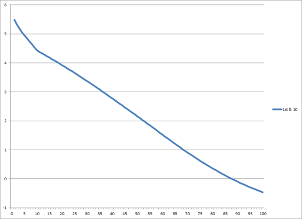
The first development of an EP model came from Carter & Machol (1971) and their work on the expected points value of 1st and 10 at various field positions. This work examined 8,373 plays from 56 games of the 1969 NFL season and binned field position into groups of 10 yards. While this is a seminal work in the field of sports analytics, it cannot be used in today’s game at any level, owing to the enormous rule changes that have occurred since (particularly the rule changes of 1974-1978 regarding pass interference and blocking restrictions (National Football League n.d.)). Their work showed, unsurprisingly, that EP increases as an offense approaches its opponent’s goal. Their data showed an x-intercept at about the -20-yard line, and a slope of about 1/14 points per yard, but with a steeper slope in the last ten yards. Carter & Machol's results are reproduced in Table 1, with a visualization in Figure 1.

Center of the ten-yard strip (yards from the target goal line): X	Expected point value: E(X)
95	-1.245
85	-0.637
75	0.236
65	0.923
55	1.538
45	2.392
35	3.167
25	3.681
15	4.572
5	6.041

Table 1: Expected Points by Field Position (Carter & Machol 1971)

Figure 1 Expected Points vs Field Position (Carter & Machol 1971)

In a later piece, they concluded that teams were far too conservative on 4th down, and kicked too many field goals where it would be more effective to attempt to make the distance to gain (Carter and Machol 1978). This conclusion that coaching decisions tend to be insufficiently aggressive on 4th down is echoed in much of the subsequent work in the field.

The Hidden Game of Football had its own chapter on Expected Points (Carroll et al. 1998). They used a linearized simplification of Expected Points, anchoring one end of the field at +6 EP, representing a touchdown, and the other end at -2 EP, representing a safety, with a straight line between them. Although later studies show this to be somewhat incomplete at either end of the field, it is reasonably accurate for the majority of situations. A reproduction of their idealized linear model appears in Figure 2.

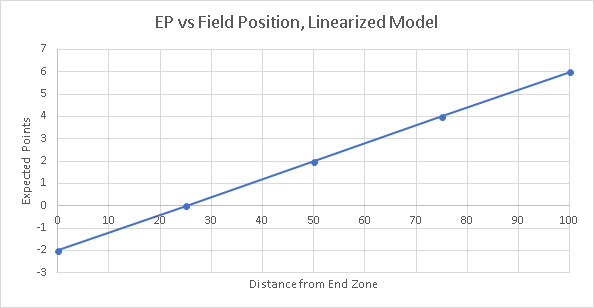Figure 2 Linearized model of EP (Carroll et al. 1998)

The idea of a linearized scoring model has certain attractive elements, and was examined by David Myers (2011). Myers work finds a linearized model to be valid between the 10-yard lines for what “response” type EP models, those that consider all future scoring. The linear assumption does not hold for similar EP-type models considering only scoring within a single drive, which he referred to as “raw” models. Raw models follow a quadratic curve, and are discussed later in this work. Myers’ comparison of the two types is included in the Figure 3.

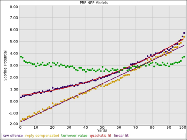Figure 3 Comparison of different EP models (Myers 2011)

The most popular work on EP is that of David Romer (2002), who created a model that used play-by-play data from 1st & 10 situations in the first quarters of games in the 1998-2000 NFL seasons, so as not to introduce end-of-half or score differential bias, while eliminating down and distance as variables. While Carter & Machol (1978) had discussed the value of kicking off and its effect on the true value of scoring plays they did not investigate further. Romer (2002) determined that a kickoff had an EP value of -0.6 points, from the average field position following a kickoff. From this he posited that a successful field goal was only worth 2.4 points and a touchdown 6.4 points.

Romer (2006) later elaborated on his work with further discussion of optimal decision-making to maximize EP and therefore scoring. Concordant to Carter & Machol (1978), Romer found strong tendencies towards risk aversion among coaches, choosing to punt and attempt field goals far more often than would be optimal. Romer’s work, benefitting from formal publication and its clear central tenets, has become the most publicized discussion of EP in the public forum, garnering 22 citations (CitEc n.d.) and broad public appeal (Dash 2010; Minkel 2008; Stromberg 2012). In a four-part series, Driner (2006a) introduced the premise of Romer’s work to an audience that may not be familiar with analytical statistics and demonstrated, through a series of examples, the notion of EP by positing a several examples (Driner 2006b). Driner (2006c) also explains Romer’s methodology while circumventing Romer’s use of jargon which, while appropriate for the Journal of Political Economy, can seem opaque to both football coaches and hoi polloi. Here Driner provides a much-needed arbiter between the common sports fan and the professional researcher.

Krasker (2005) demonstrated mathematically that near a game’s beginning, the win probability function becomes sufficiently smooth that it can be considered linear over a small range of score differentials. This justifies the use of EP as a decision-making tool in most game situations, avoiding the need for computationally expensive Win Probability models that in 2005 remained at the very limit of both computing power and available play-by-play data. Krasker (2004) also created a decision-making engine that incorporated EP concepts into its dynamic programming model. Albeit nominally publicly accessible and open-source, Krasker’s documentation is jargon-heavy and written in MATLAB, both factors that would limit public interaction. Krasker cites both Carter & Machol (1971) and Romer (2002) as being purer EP models, whereas his model incorporates WP elements.

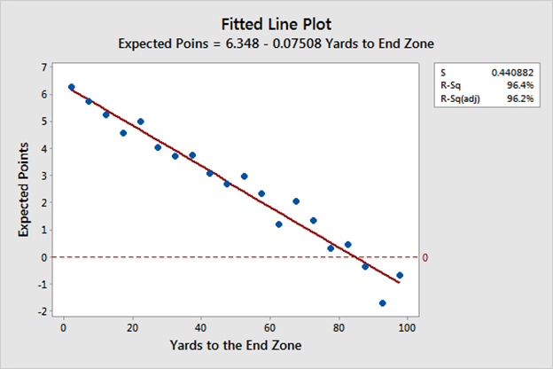
An EP interface first reached the public with the model developed by ProTrade (Kerns et al., n.d.), a fantasy sports site, and was later used by ESPN. While now defunct, it served as a direct inspiration for Burke’s (2008b) model that is now used by ESPN. Burke (2008a) created his model of Expected Points to develop on prior work. His conclusions follow others showing EP to be linear in the middle section of the field, between the 10-yard lines, but tailing toward either end zone. Burke’s figure for 1st down EP is included in Figure 4. Burke (2009b) would later publish his results for EP across all down, distance, and field position states. Burke also demonstrated continuity between the EP and P(1D). Since P(1D) of 2nd & 5 is approximately equal to P(1D) for 1st & 10, we should expect and in fact do see that EP for 1st & 10 at yard line X is roughly equal to EP for 2nd & 5 at yard line X-5.

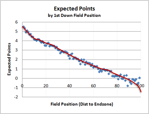Figure 4 EP values by field position (Burke 2008a)

In keeping with Romer’s (2006) determination of touchdowns and field goals being worth less than their nominal value, because of the ensuing kickoff, Burke (2008d) also discussed the value of a safety. Safeties are unique in that the team that scores also receives the following kickoff, and that the kickoff for these occurs from the -20. Given the excellent field position that usually results from receiving a kickoff that is kicked 15 yards behind the usual kickoff spot, Burke estimates a safety to be worth 3.6 points, as the ensuing position is worth an additional 1.6 points to the 2 nominal points of the safety.

The question of the value of a score is central to the development of any EP model. To assess the value of a touchdown, there are two important considerations. First, one must consider the nominal value of the touchdown. This is about 6.98 points, given the average conversion rate of extra point attempts and two-point attempts (Romer 2006). Then we must consider the subtracted value of the kickoff and subsequent possession. This is calculated by taking the EP value of the average starting position after a kickoff. However, this method is not complete, as we have altered the value of scoring plays, such that a touchdown or field goal is now worth less than it was when we made our first calculations, and a safety is worth more, in that it has a greater absolute value. It becomes necessary to recalculate our EP curve with the new scoring values, and so on recursively until we converge. Only Goldner (2011e) explicitly states the use of this recursive methodology. Whether a recursive method produces noticeably different results remains to be seen.

As her Master’s thesis, Wright (2007) did a comparative analysis of EP-based 4th down decisions of 5 NFL teams in the 2005 season. Wright’s model only uses a raw model of EP, and while it attempts to compare both EP and P(1D) across teams it suffers from very small sample sizes even after binning field position and the value of the study as a means of comparing teams is not much more worthwhile than simply looking at their records.

In their comparison of applied decision-making to game theory in football and baseball, Kovash & Levitt (2009) developed an EP model of 2001-2005 NFL seasons with n=127,885 to compare the expected utility of runs versus passes, finding that offenses run too often. Their EP model uses a different methodology, focussing on total Net Expected Points over the entire half, but the conclusions are compatible with other models. Their model is unique in its incorporation of interaction terms, while their results do not show the dip in EP when an offense is backed up to its own goal.

Gallagher (2011) expanded on the work of Romer (2006) by using a much larger dataset, with 430,022 plays over 10 years of NFL play; Gallagher used 1st & 10 plays from his dataset, without restricting himself to 1st quarter plays as Romer did. This decision has both beneficial and harmful effects on the validity of the results. For instance, end-of-half plays may skew the data where teams must make short-sighted decisions to score urgently, or alternately may be willing to concede not advancing the ball in order to end the half without giving the other team the ball. Score differential may come into play as well, teams trailing or leading by large margins stop behaving typically and are more willing to either concede points or take greater risks. Conversely, most of football does not occur in these situations; some of these problems will tend to offset over a larger data set, and on the balance the increase in sample size and the resultant reduction in error may be more helpful than harmful.

A rarity in football analytics, Monte McNair (2011a) developed an EP model of college football using over 1,000 games of Division I football, both FBS and FCS subdivisions, from the 2010 season. This model defines touchdowns as being worth 6.3 points and field goals as 2.3, consistent with Burke (2008a) and Romer’s (2006) work on NFL EP. This curve, included in Figure 5, is also flatter than the NFL curves described above, a team backed up to the -1-yard line is still only at -0.5 EP, and the curve peaks at 5.5 EP.

Figure 5 EP vs field position for NCAA football (McNair 2011a)

Although McNair’s (2011a) analysis provides no discussion on the difference between his NCAA model and NFL models, we can infer from the flatter curve that field position is less relevant in college football; an offense’s chances of scoring are less dependent on field position. Thus, college football would seem to be subject to more influence from long scoring plays. The McNair model also does not have a tail when the offense is behind the -10-yard line, consistent with the position that college football has more long scoring plays and that field position is relatively less important.

A college football model based on Big Ten conference games in 2013-2014 (Rudy 2015) found higher EP values than McNair’s model (2011a). Because of the limited dataset this model binned data by field position into 5-yard increments, and so does not show the tailing towards either end zone, as shown in Figure 6. This model did separate by home and away team, demonstrating that home field advantage is worth about 0.6 EP across all states.

Figure 6 EP vs field position for Big Ten football (Rudy 2015)

Pro Football Reference (PFR) (Mike 2012) created an EP model to augment their encyclopedic database of information, especially their play-by-play data library. Although their model remained proprietary, it was criticized after reverse-engineering (Myers 2012), since the results that emerged were inconsistent with the results of any prior work in the field. In particular, as an offense approaches the goal line, the PFR model used deviates from other results in the field, showing an EP value far too high and lacking what Myers refers to as a “barrier potential.” The barrier potential is the difference between the highest EP value in a model and the value of a touchdown. Viz., PFR’s model gives a maximum EP value of 6.97 for 1st & 10 at the +1, and values a touchdown as 7 points. This itself a debatable point, as touchdowns are only worth 7 points very late in a half, as originally postulated by Romer (2002). The implication is that the probability of scoring a touchdown from this scenario is greater than 99%, a number not corroborated by other works of EP or P(1D). Given the proprietary nature of the model, the cause of this result is unknown, although it is suspected to be an effect of a fitted function (Myers 2012).

Causey (2015a) used 14 seasons (2000-2013) of NFL data to compare EP over time. By separating EP curves by season he showed a general increase of approximately 1 point of EP over the span of the study. This implies a general increase in scoring across the league, and one attributable to more successful long drives (Causey 2015b). Causey notes his statistical methods in detail, particularly his use of bootstrapping as a smoothing device – shown in Figure 7 – in comparison to Burke’s (2008a) preference for local regression. Causey also makes some mild critique of Burke’s failure to note variance in his outcomes, especially when using this information to inform a 4th down decision. Causey’s concern is the implication that a 4th down decision can be reduced to one choice being objectively better, when in fact the decision is probabilistic, the result of three overlapping EP distributions, reiterating the prior comments of Lopez (2013).

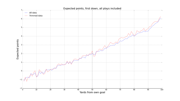Figure 7 EP vs field position (Causey 2015a)

As NFL data is now digitized, we can expect incremental improvements in models as we have the ability to become restrictive with the parameters without compromising our confidence in the results. Burke (2012) did assess the growth in EP over short timespans, and we can expect to see developments on the historiography of EP as more data becomes available. Causey (2015a) came to similar conclusions on the changes in EP.

While most EP efforts develop the raw data and then place fitted functions, a more involved method involves modelling the game via a Markov method. By identifying all the potential game states and the relationships between them we can determine the probabilities of transiting between any two states (Goldner 2011b). Classifying plays by down, distance, and field position can show how a drive is most likely to proceed until what is known as an “absorption state,” when a drive comes to a conclusion (Goldner 2011c).

Markov models allow, in principle, for a complete model of all possible outcomes of the game, and a calculation of the probability of any outcome. This is a common approach to baseball modelling, since each transient state can only lead to a limited number of other states, and the datasets are much larger. Markov models of baseball are thus fairly common (Bukiet, Harold, and Palacios 1997; Hirotsu and Wright 2003; Sueyoshi, Ohnishi, and Kinase 1999).

Krasker (2004) used Markovian elements in his dynamic programming model, while Goldner (2011d) developed the first fully Markov-driven model. A limitation of the Markov approach is that it requires binning similar states, as Markov models do not respond to states that are empty or have very few elements; the number of states in an EP model is on the order of 104, with some being very rare.

Unfortunately, football WP models by Markov methods are not practical for want of data, but they do prove useful for EP models. Goldner’s (2012a) model begins by simply determining the probability of each absorption state – each possible way of ending the drive – as previously discussed by Burke (2009). Goldner (2012b) later included the likelihood of the drive continuing for any n further plays.

A variation on EP is the notion of “raw” EP, considering only the points scored within a drive. These models do not look forward to subsequent possessions; as a result, negative points can only be scored via safeties or defensive touchdowns, making a negative EP value almost unheard of. Since most drives do not score points, this leads to all plays on those drives being scored as 0, compressing the entire EP curve toward 0. The most thorough of these was developed by Goldner (2011e). His work shows no cases of negative EP for 1st & 10 regardless of field position, with negative values only in extreme cases. While response-type EP models such as those discussed above are linear between the 10-yard lines, Goldner’s raw model is quadratic over the length of the field as shown in Figure 8.

Figure 8 Raw EP vs field position (Goldner 2011e)

Goldner’s (2011e) raw model evolved into a recursive model (2012c), subtracting the EP value of punts and turnovers from each state’s EP. This was treated recursively until an equilibrium was found (2012c). These results show different values from other models when nearer to one’s own goal line because the average value of all punts and turnovers is used rather than the average value of punts and turnovers from that field position.

Alamar (2010) used a set of 220,326 plays from the 2005-2008 NFL seasons to create a raw EP model to assess the marginal outcome of plays by measuring “NEP,” Net Expected Points. This concept, also referred to as Expected Points Added (EPA), is the change in EP over a play. Alamar (2010) also separated passing and running plays, with the conclusion that passing plays have a higher average NEP and a higher probability of a positive NEP, arguing that, in general, passing is a superior option in the current game. Alamar does not go into the second order game theory aspects of this implication, and the effects that a shift in offensive playcalling would have on defensive strategy.

Burke (2009a) critiqued Alamar’s work, albeit prior to it having been formally published and on the basis of its presentation at the New England Symposium on Statistics in Sports. Burke’s criticism is particularly pointed at Alamar’s regression methods, specifically the use of a linear regression for EP values. Burke was also critical of any EP models failing to consider quarter and score as context, and he advocates for similar restrictions to those used by Carter & Machol (1978) or Romer (2006). Finally, he disputes Alamar’s assertion that EPA can be viewed in binary terms as either being positive or negative.

Prior to building his response EP model (Rudy 2015), Rudy (2012) developed a raw model which also shows a quadratic relationship between field position and points scored. This model only uses starting drive position, and uses 3rd down conversion rates as a proxy for 4th down conversion to show optimal decisions for each situation. Because this data only includes drive starts, the resolution is limited and data is binned into 5 or 10-yard increments, as shown in Figure 9. There is no discussion as to whether 1st & 10 plays at the start of a drive (P&10) are meaningfully different from 1st & 10 plays later in a drive.

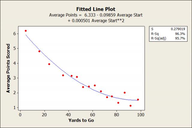Figure 9 Raw EP vs field position (Rudy 2012)

Another raw EP model of college was consistent with the quadratic relationship to field position seen in NFL studies (Justin 2013). This model treated offensive and defensive raw EP separately. Although defensive raw EP never rises above 0.5 points, It demonstrably jumps at the -5 yard-line. Unfortunately, without better discussion of confidence intervals the meaning of these values is difficult to determine.

These raw models fail to consider the long-term effects of field position. While no points may be scored on two different drives, the resulting field position can have a significant impact on the opponent’s scoring chances. While statistical analysis almost always encourages coaches to go for it more often and punt less, Rudy’s (2012) recommendations are much more aggressive than others.

Though not replication studies, EP models have demonstrated consistent results. Starting with Carter & Machol (1971, 1978) we see the same general results, as Causey (2015a) hews closely to Gallagher (2011), who hews closely to Kovash & Levitt (2009), and to Burke (2008a), Krasker (2005), and Romer (2006). Among models using actual play-by-play data, vis-à-vis the linearized model of Carroll et al (1998), the only dissident voice is PFR (Mike 2012), whose model is proprietary and cannot be compared to the others. Researchers who show an open methodology have seen their work ratified. Although there can be some discussion of the merits of different techniques, such as the parameters by which data may be included or the statistical smoothing techniques, there appears to be a solid consensus in the field regarding the EP value of field position. Id est, EP is generally linear between the 10-yard lines, with a steeper slope at the ends of the field. This supports traditional football wisdom that the marginal value of yardage near either goal line is more valuable than in the middle of the field.

While attempting to develop a means of evaluating individual players independent of the contributions of their teammates, Yurko et al. (2018) developed a novel EP method by using multinomial logistic regression to create estimates of probabilities for the next score, from which they could “trivially estimate expected points.” The largest benefit to this method is that it better accounts for the small sample sizes that are often found across the thousands of bins. Using data from 2009-2016 and 304,896 plays. This study is also the most thorough in its methodology, including calibration graphs for each scoring event.

Curiously, Yurko et al. (2018) choose not to adjust the value of each scoring event, leaving each at their nominal value (7 points for a touchdown, 3 points for a field goal, 2 points for a safety) and not accounting for the ensuing change of possession. Conversely, rather than directly calculating field goal success probability they use a generalized additive model. While such a model is useful at longer ranges where sample sizes shrink, it seems excessive at shorter distances where there is more than enough data to accurately determine the probability of converting a field goal attempt. Ultimately, in spite of their more sophisticated methods of developing a model, their actual results show very similar results to most of the other work in the field. EP changes in roughly linear proportion to field position until about 15 yards from the end zone, at which point the slope of the curve steepens sharply.

Looking at these studies chronologically, one sees the development of the personal computer and its use in statistical research. While Carter & Machol (1978) worked with n=8,373 and presumably did calculations by hand, Romer (2006) had n=11,112. The development of larger datasets and cheap computers to handle said data between 2003 and 2010 allowed Alamar (2010) (n=220,326) and Gallagher (2011) (n=430,022) to work with a data set an order of magnitude larger. Although Gallagher used less stringent restrictions on which plays to include and Alamar examined states outside of 1st & 10, this is tied to two key concepts: first, that NFL data was not digitized prior to 2000, and second, that personal computers of an earlier era could not have handled such massive datasets. Calculating EP by hand with a six-figure dataset would have been an impossible task for Carter & Machol (1978).

As EP models have grown to include more than just 1st & 10 states, the emergent discovery that 2nd & 1 is more valuable than 1st & 10 has come forth. The working understanding is that this provides the offense with a free play to attempt a large gain downfield, since an unsuccessful play results in an easily converted 3rd & 1. EP and P(1D) imply that the offense actually has two free plays, as the offense should usually attempt to convert 4th & 1. This effect was first discussed by Burke (2008c), with further mention from Birnbaum (2008). Although the incidence of nine-yard gains on 1st & 10 is significantly greater than the incidence of 8-yard or 10-yard gains (Burke 2008c), this is likely a product of the rounding issues discussed earlier (N.B. the rounding is actually done with respect to field position, so as to reconcile play-to-play, but this approximation will suffice for demonstration). McNair’s (2011b)model showed the same result in college football, as he analysed the marginal value of yardage in the context of fumble rates.

4 - Conclusion

The strongest criticism of EP models is in the handling of the statistical methods. Causey (2015a) uses an example showing the change in EP over time to explain how EP models can fail to accurately describe the present game. Hermsmeyer (2016) showed the effect of noise and small samples that occur when creating unique EP values for all down and distance combinations. Regression for situations other than 1st & 10 show poor fits, and smoothing techniques have very wide confidence intervals. For some rarer combinations of down & distance the scatterplots are so noisy as to be unintelligible. Future work on EP will likely focus on improved precision regarding the EP values of given states and the value of scoring plays, ongoing investigation into the growth of EP values over time. Perhaps most importantly, future work will likely seek a better understanding of how individual teams affect EP curves, especially whether all teams are slight variations of the general curve or if different teams have unique EP functions.

From a methodological perspective, understanding the nature of error and confidence for EP is an area of future study, especially given the unusual structure of the data. Understanding the confidence intervals of EP values will allow for better estimates in decision-making, and a more nuanced understanding of optimal gameplay. Areas of study might include the use of P(1D) to normalize non-1st & 10 states to an equivalent 1st & 10. Alternately, research into which similar states can be binned might allow for large enough sample sizes to determine EP with greater confidence. It is hoped that EP can be used to improve decisions, but this will itself have a significant effect on the EP function; the future of EP will necessitate updating existing models as coaching decisions evolve.

While EP models could always use more data, we must consider the cost of including this data. EP is changing over time (Causey 2015a), raising the issue of how much historical data can be justified. As we reduce statistical error in using more data, we also introduce systemic error. As EP increases over time as a result of improved passing games and rule changes, improved 4th down strategy will also cause further increases. The associated increase in P(1D) will also have an effect on EP. Such changes in EP will require the recalculation of 4th down charts and careful consideration of which data to include in an environment where both EP and P(1D) are in flux. From an applied perspective, EP can be considered the most interesting of the models, as it lies at the intersection of high confidence in results, easy application in a majority of game situations, and having a significant impact on the game’s results.