1-Abstract
The conclusion of a three-part series discussing the three major fields of research in American football analytics; First Down Probability (P(1D)) (Clement 2018a), Expected Points (EP) (Clement 2018b), and Win Probability (WP). This chapter discusses the existing body of work regarding WP and various models derived to estimate it over the last 30 years. Development in the sophistication of model-building techniques is an ongoing theme, and better understanding of measures of uncertainty are an emergent topic as competing models enter public view and analytic notions infiltrate the sporting lexicon.
2-Introduction
The most all-encompassing of football analytics models is the Win Probability model. These models give a probability that a team will win a particular game, given a game state. The state variables involved include score differential, possession, field position, down and distance, timeouts, and time remaining. The most developed of these models make allowances for home field advantage and relative team strengths. While WP alone is prone to significant variance, the more applicable use of WP is the notion of Win Probability Added (WPA). This is the difference between two states, generally consecutive plays or over the length of a drive. WPA can also be used for decision-making where the expected outcomes of the different options are compared.
In contrast to EP, WP is context-sensitive. Maximizing EP is not always an appropriate strategy, especially towards the end of the game. In principle, all decisions should be made in the context of WP, and not EP (Jokinen 2017). WPA can allow us to consider the utility of strategies that may lead to negative EPA values but positive WPA values. Burke (2010) gives an example of whether a team that is leading and trying to run out the clock should risk passing the ball for a game-clinching first down, or run the ball and likely punt but with less time remaining.
Early in games, EP and WP are compatible concepts, as Krasker (2005b) demonstrated. EP models are preferable for early-game decisions; they offer greater confidence since they do not consider certain important contextual variables, such as score and time remaining. However, late-game decisions are best left to WP where this context becomes more important.
3-Win Probability
An early investigation of win probability involved using pregame point spreads as a proxy for team strengths and determining win probabilities based on these lines (Stern 1991). Final score differential was found to be a normal random variable with a mean of the Vegas spread and a standard deviation of 13.86. This gives us a pre-game estimate of each team’s chances, but does not allow us to determine the change in win probability as the game progresses. Stern’s work is influential in providing a framework for team strength-adjusted WP models. The work of West & Lamsal (2008) includes a detailed literature review of game prediction research, with a focus on pre-game information to make outcome estimates.
The consideration of in-game situations was not approached until Krasker (2004) who was able to reduce the problem to a set of equations that could be used to determine one’s WP under any conditions. Krasker used a Markov model to create a backward induction-based system. Working in the last two minutes of a game, Krasker (2005a) presented more specific WP estimates for the last two minutes of the game in 30 second intervals, based on score differentials of <3, 3, and >3. Most importantly, he accounts for how many timeouts the offense has remaining. This information allows a team to make an informed decision on the impact of using a timeout to stop a running clock.
The now-defunct ProTrade (Kerns et al., n.d.) used a similar backward induction process to determine optimal decisions. This model was eventually used by ESPN before being shuttered in 2009. Another defunct model was built by Gridiron Mine (Freeh and Lowenthal 2007), called the Victory Forecast. The model also included the Whether Station, intended as a resource for analyzing decision-making. Abandoned in 2010, the model is no longer functional, but its logistic regression method inspired a piece by Driner (2008), where he developed a rough outline of another logistic regression model. While incomplete, Driner’s model is the first known instance of teams being given nonequal initial win probabilities. The model does not go into the fourth quarter and is left skeletal, as three functions – one per quarter – based on score differential, initial team strength, and home field advantage. It also unfortunately gives no indication of methods or confidence.
Starting what would become the flagship of WP models in 2008, Brian Burke (2008) made a WP model using play-by-play data from 2000-2007 NFL games. This model would eventually replace the ProTrade model at ESPN, which had provided Burke with his initial inspiration. Rather than using the analytical methods of his predecessors, Burke used a more direct calculation of WP, by averaging the outcomes of states similar to the one in question, binning plays of similar type across different variables. Burke’s (2009a) model has grown to include several factors, such as a logistic regression to determine initial team strength by weighting various independent factors proportional to their correlation with winning (Burke 2009b). A later version better accounted for endgame situations and was updated in response to the style of play seen in the NFL (Burke 2014). Burke (2009c) also released a calibration graph of his model against 2008 data, included in Figure 1, plotting predicted WP against true WP for bins of predictions rounded to the nearest percentage point. A calibration graph involves plotting predicted WP against the actual win proportion and comparing it to the ideal line where predicted WP equals true win proportion – that is, when the model predicts a WP of 75%, that team goes on to win 75% of the time.

Figure 1 Win probability calibration graph (Burke 2009c)
A model based on logistic regression created on the Wolfram Alpha architecture, using “over 110,000 in-game situations from 2006 to 2008” (Prince 2011). This model allows the user to define the game state receive the WP in return. Unfortunately, although Prince’s code is publicly available, this is only a forward-facing interface without the training data; the coefficients of the logistic regression are all that is visible. Logistic regression as a means of calculating WP would prove a popular approach in later years.
Seeking to develop a model with a clearer understanding of its own uncertainty, Causey (2013a) worked to develop a model that produced results more nuanced than prior efforts. Using data from the 2001-2013 NFL seasons (Causey 2013b), he developed his model with random forests (Causey 2013c) to incorporate measures of confidence and uncertainty into the WP model. Random forests are beneficial in this context because of their ability to handle multiple non-linear interactions between the explanatory variables. More so than previous models, Causey (2013a) describes in detail his methods and uncertainty of his model, highlighting the limitations of both creating and testing WP models. The model includes terms to incorporate the Vegas line before performing validation checks on the test data set (Burke 2014). These calibration tests are included in Figure 2 and show that the error in Causey’s model is generally toward the extremes. That is, low “true WP” situations tended to show an even lower WP, and high true WP showed even higher.
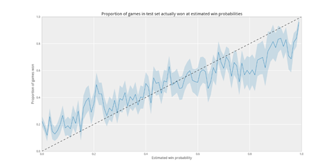
Figure 2 Win probability calibration graph (Causey 2013a)
Certain characteristics of football have proven difficult to model. Timeouts, for instance, have minimal impact on WP until very late in the game, when they become tremendously important. A leading team can also choose to kneel out as much as two minutes of the game. Causey (2015) also writes at length about overfitting and bias-variance trade-off. Most models calculate win probability and then pass through several additional steps to catch discontinuities, such as when kneel-outs are viable, or when teams have an option to kick a field goal at the end of the half (Causey 2015). Attempting to capture each of these scenarios is not practical, but the alternative is to continue adding features to the model ad infinitum. A model that perfectly describes its test data will also capture the random error in the test data, an error that will not be reproduced the next season.
Borrowing heavily from Stern (1991) and Winston (2012), a new WP model for Sports Reference was built through a collaboration between Lynch (2013) and Paine (2013). Knowing the expected final score and its variance, they weighted this across the length of the game. After accounting for team strength, the Sports Reference model incorporated down, distance, field position and possession by using EP. EP can be accurately calculated, since there are orders of magnitude fewer states than for WP. Applying the expected scoring distribution determined above and shifting according to the current score differential and the current EP gives a normally distributed expectation of final score differential (Paine 2013), from which one can calculate WP by using a one-sided t-test. The Sports Reference model is exceptionally simple, and it can be calculated with only a high school level understanding of statistics – mean, standard deviation, and t tests. Unfortunately, it does not include certain important modelling features. Without including the timeout state, late-game decision-making cannot be made with this model. The most perilous assumption is that scoring is a continuous affair, rather than something that occurs in discrete chunks. While this model should provide reasonable results in the early part of the game, in that case we can just use EP alone, following Krasker (2005b).
Inspired by Burke’s (2008) work, Lock & Nettleton (2014) developed a WP model using random forests on 2001-2011 NFL data in a similar manner to Causey (2013a). They tested this method against 2012 NFL data. Their results are consistent with Causey’s in terms of uncertainty. Several variations on the model attempted to improve performance, but increasingly complex methods did not yield better results. The authors considered their outcomes to be similar to Burke’s, providing better results at the beginning of the game. It should be noted that the comparison is to Burke’s first model and not his later model (2014) which more accurately reflects differences in team strength.
With the development of betting exchanges, which allow gambling contracts to be made at any point in the game, there is an enormous financial incentive to develop accurate in-game WP. NFL gambling is a $95 billion annual market (American Gaming Association 2015), so an effective predictive model would provide the same kind of advantages that financial algorithms had for traditional markets. Gambletron 2000 (Schneider 2014) is a WP model designed with the intention of facilitating these bets. Using the standard features, Gambletron 2000 was developed to find and exploit inefficiencies in gambling markets (Schneider 2014). As a result, their methods remain proprietary and cannot be compared to the others discussed here.
In an astonishing demonstration of scope creep, Benjamin Soltoff (2016) set out to determine the value of a timeout and finished by developing a random forest WP model. Ranking features by their Gini Importance showed, unsurprisingly, score differential to be the strongest determinant of WP, with point spread, time remaining, and field position also ranking highly. Soltoff’s calibration graph, shown in Figure 3, showed the same weak points in the extremes as Causey (2014). Unfortunately, Soltoff was unable to adequately determine the WP value of a timeout.

Figure 3 Win probability calibration graph (Soltoff 2016)
Hoping to foster openness in the community, Andrew Schechtman-Rook (2016) created an open-source WP package. He mentions the obscurity of models developed by Burke (2014) as well as other less popular models. While he mentions Lock & Nettleton (2014) as being the most open of the models, their code is still inaccessible. The PFR model has a clear and published methodology, but Schechtman-Rook (2016) notes two significant flaws in their model. The structure of the model makes it susceptible to issues regarding the validity of EP as a proxy for WP late in games, and the model shows very discontinuous jumps that lead Schechtman-Rook to question whether it is “buggy” or “pathologically incorrect”. Schechtman-Rook (2016) argues that the lack of transparency in sports analytics makes much of the work in the field irreproducible. Furthermore, it cannot be effectively verified. A calibration graph of the Schechtman-Rook’s model can be seen in Figure 4. While calibration graphs are not proof positive of quality, they are the easiest “at a glance” measures of a model’s predictive accuracy, albeit at the risk of overfitting, as was discussed by Causey (2013a).

Figure 4 Win probability calibration graph (Schechtman-Rook 2016)
A college football model employed a novel approach in determination of WP (Moore 2013). An initial prediction of team strength is based on various performance indicators from previous games. Factors from current-game performance relating to offensive and defensive efficiencies are then added. Score differential and current Expected Points are also factored into their calculation. The relative weighting of each factor is adjusted based on the time remaining in the game. Although the model is “a bit of a hack” (Moore 2013), the model does have a calibration coefficient of 0.940, albeit with a tendency to overstate WP.
A logistic regression-based model of 2009-2012 NCAA football games (Mills 2014) and tested against the 2013 season gave a similar calibration graph to Moore (2013), included in Figure 5. All models, NFL or NCAA, with available calibration graphs struggle to accurately predict extreme outcomes. Also, the time remaining in a game is a rather complex feature, since the team with possession has a number of options available to extend or shorten the game by using different tactics. Therefore, the effective time remaining late in a game may have more to do with which team has possession than with how much time is actually on the clock.

Figure 5 Win probability calibration graph (Moore 2013)
Given the recent high-profile comeback during Super Bowl LI, the issue of model accuracy at extremes has drawn increased interest. The Patriots’ win probability was given at less than 1%, and yet they prevailed. In the aftermath of the event, Lopez (2017) compared various models – most of them also discussed here –and compared them across the game. Cross-correlations across each pair of models gave r2 values between 0.45 and 0.85. It is perhaps concerning that a number of generally well-calibrated models do not relate cross-correlate well. The work concludes with a list of five recommendations for WP models, mostly relating to validation and acknowledging the uncertainty in each model.
Super Bowl LI also prompted discussion from Konstantinos Pelechrinis (2017) as he presented his own model. This model used 8 seasons of NFL data in a logistic regression model (Pelechrinis 2018) with a calibration coefficient of 0.99, demonstrated in Figure 6. This work was published in a working paper (Pelechrinis, 2017), and an end-user interface is also publicly available (Pelechrinis 2017a) where users can define a game state (Pelechrinis 2017c). Forward-facing interfaces allow the public to interact with analytics and promote an understanding of the goals and methodologies of analytics.

Figure 6 Win probability calibration graph (Pelechrinis 2018)
Although it is possible in theory to put all football decisions in terms of WP, it is often impractical to do so because the specificity of each state limits the amount of data available for each state, even with smoothing across similar states. The application of different smoothing techniques can also significantly impact the results (Lopez 2017). WP models are known to not be robust in the extreme values, and similar models can have greatly varying odds ratios. A more universally useful application of such models is the use of WPA. The marginal WP over a play is much less susceptible to these problems at extremes and is valid for influencing decisions.
The problem of inadequate datasets is somewhat intractable. Even a model that considers only field position, time remaining, and score differential will have millions of different states, and a football game only produces about 200 data at the upper limit. An entire NFL season gives us around 50,000 data, and 10 seasons gives us 500,000. As the game continues to evolve, it is unrealistic to use data more than a decade old, as it will be a different game played under different rules. For NFL WP models we are restricted to using statistical methods to bridge the gaps in our data.
College football WP may offer some opportunities for WP, as there are triple the number games played at the FBS level; if we include lower divisions such as FCS we may get as many as 7 times the data of an NFL season. While the results of such a model could not be directly applied to the NFL, it would allow for testing of different data management techniques that could be applied to NFL models.
WP models can be said to be accurate in the aggregate, but have fairly large variances on each individual play. They are not generally robust in terms of odds ratio at their extremes, but the precision is adequate for making in-game decisions based on WPA. These tenets hold broadly true for the various major families of WP models – smoothing, random forests, backward induction, and logistic regression.
Win Probability models with calibration graphs available give a good sense of where football analytics stands. r2 values of all known calibrations are all >0.9, with some >0.99. Late-game situations are a known source of consternation for WP models, especially with respect to timeouts and game-winning field goals. The models are very noisy at the extremes. By looking at odds instead of probabilities, it becomes clear that even two well-calibrated models can show extremely different odds for the same situation.
Many WP models use multiple logistic regression. While in application this has proven to be effective, it makes the assumption that all factors involved are constantly weighted, a concerning thought. A prima facie example: in the final minute, field position is not at all important when leading by any margin, but critically important when trailing. To some extent it is possible to code for these eventualities, especially for kneel-out situations, but it is not reasonable to handle all of these manually. A suggested investigation would be to create multiple WP models of the different types (logistic regression, random forests, backward induction, etc.) and to run comparative calibration tests on each to compare the efficacies of different models.
Figure 1 Win probability calibration graph (Burke 2009c)
Figure 2 Win probability calibration graph (Causey 2013a)
Figure 3 Win probability calibration graph (Soltoff 2016)
Figure 4 Win probability calibration graph (Schechtman-Rook 2016)
Figure 5 Win probability calibration graph (Moore 2013)
Figure 6 Win probability calibration graph (Pelechrinis 2018)


No comments:
Post a Comment