It's a Game of Field Position: Punting in U Sports Football

1. Abstract

An analysis of the objective measures of punting in U Sports football,. This work looks at gross, net, and EP values of punts by yardline and compares them to one another. All measures are shown to have cubic fits. Punt spread is also examined as the difference between gross and net punting. Punts are heavily compressed with decreasing yardline below 50 yards, and conversely increase significantly in value with increasing yardline above 90 yards. While the first of these is expected, the second is unexpected. Further research is necessary, with the preliminary hypothesis that it stems from a selection bias of only teams that punt well choosing to punt from those situations.

2. Introduction

While punts have been maligned by much of football’s analytic corpus, there is still undoubtedly a role for the occasional punt in a game. Even the most polemic of works supports this notion. To date, most of this work has been focused squarely on the NFL (Clement 2018b), with some limited works looking at CFL data (Clement 2018a). No known works discuss punting in detail in a Canadian context, nor of punting at all in U Sports.

What is presented here is three forms of measuring punts. Ceteris paribus, each of these measurements is “good.” Id est, put that has a greater gross yardage is generally better than one with lesser gross yardage, but this is, of course, only a very rough measure. Net yardage is nearer the truth, as a punt with better net yardage is strictly better than one with worse net yardage, but the process to achieving this net yardage must consider risks and benefits of such decisions. Expected Points (EP) can be used as a still-more refined measuring stick that, with the exception of Win Probability-dominant situations, can assess the value of a punt, but is still an incomplete measure given the greater variability of punts relative to ordinary scrimmage plays.

3. Punting

While the simple matter of measuring a punt’s yardage is a straightforward task, measuring its value is far more difficult. Punts may be one of football’s more intractable questions, for while it carries all of football’s usual variables and context, these are generally tempered by the very team-oriented nature of the sport that limits the impact of any individual player. Field goals, conversely, can largely be modelled as a single man against the fates, and so we can isolate him from all the other players, whose performances are comparatively insignificant. Punts, however, have a punter with disproportionate impact, and his performance directly plays into the other players on the field. The returner also has an outsized impact, and his abilities, real or perceived, can then impact meta-decisions about whether to punt “true,” that is to say, long and high and far, or whether to attempt a strategic gambit to punt directionally, or even out of bounds entirely. While opponent strengths and weaknesses always have an effect on a football team’s decisions, the focus on a single player creates large variance in the outcomes.

a. Gross Punting

To properly assess punting is a difficult task, to be sure, but it must begin with the basic measurables., the first of which is the gross yardage of the punt. This is simply the distance from the line of scrimmage to the point where the ball was first recovered. Although this number alone is only a very rough estimate of the punt’s value, as it neglects any information on hang time or placement, and the effects of field position, it is a first-order measurement. Gross punt yardage was determined for punt plays where possible. Most punts in the play-by-play data note the gross yardage of said punt, and through string comprehension this value could be save to the play object. Each punt object could then hold an array of all the gross punts from a given yardline. Confidence intervals were determined by bootstrapping this array, using 1000 bootstrap iterations. While we only look at punts with N>100, a number which should be suitably large to look at the distribution directly, bootstrapping offers certain advantages:

1. Consistency: Bootstrapping has been the method of choice within this corpus, as it was necessary to determine intervals for certain highly non-normal and discrete distributions, such as when determining EP values (Clement 2019).
2. Non-normality: Even with a large  sample of punts the distribution is unlikely to truly be normal. Gross yardage is upper-bound by human performance at about 50 yards, even with friendly winds and bounces the right tail is going to be significantly curtailed. As we approach the end zone gross yardage will be capped at the goal line, further impacting the distribution. When later looking at net punts, the left tail is going to show a spike at the value of the starting yardline, the result of punt return touchdowns. Once a punt returner evades the coverage unit her is rarely stopped just shy of the goal line, compared to the number of punt return touchdowns. Applying a normal distribution to gross punting would be, at best, a first approximation.

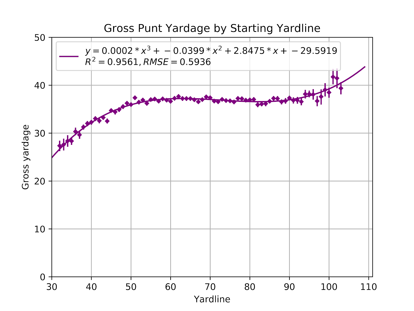
Figure 1 Gross Punting Yardage by Starting Yardline

Logically, gross punting should be upper-bound by yardline, notwithstanding the rare punt that is returned from within a team’s end zone, and lower-bound at 0 yards, notwithstanding the very rare negative punt. Once the compression effects of the opposing end zone disappear around the 50-yard line, there should be no effect from field position, the punting team is unconstrained. While we doe see this for the bulk of punts in the midrange of the field, we also see the fitted curve rising as of about the 95-yard line. There is no reason that being deep within one’s territory should make a given punter more capable of punting the ball farther, but it seems more likely that there is a self-selection bias at play, that teams who have excellent punters are the only ones choosing to punt from their own end zone, where most teams are likely to conceden a safety. Whether either of these teams are justified is a question better answered by a well-developed EP model than by simple gross yardage. If these could be effectively removed from the sample then we could expect to see a flat line for punts beyond the 45-yard line, and the better fitted function would likely be an exponential function that runs asymptotic to the flat line of data points. This curve would likely fit a better theoretical expectation, passing near the origin, as opposed to the current y-intercept of -29. In practical terms this isn’t particularly meaningful, there is never going to be a significant number of punts from the red zone, but it is preferable to have an estimated model that can be extrapolated.

And yet, such a model may simply prove unnecessary. Note that for most of the data points the error bars are not visible. This is not due to them being omitted, but rather because they are so small as to be subsumed by the data point itself. In order for this to occur the 95%CI must be within about 1 yard +/-, given the size of the data points. There are some implications from this. The average values can be used as more than simple means, they can be treated as point estimates with negligible variance. This also implies that U Sports punters are remarkably consistent both from punt to punt and from punter to punter

b. Net Punting

Net punting for each punt was determined by the difference between the yardline of the punt play and the yardline of the subsequent play, adjusted for possession. By design, this includes all the things that could happen on a punt play, including penalties touchdowns, and fumbled returns recovered by the kicking team. Most importantly, rouges are taken with a net from the yardline of the punt to the 35-yard line spot. Net punting here does not seek to evaluate the “goodness,” of a play, it is merely the net yardage exchanged on that play. A long return that ends in a fumble will still show as a negative value. Determination of the goodness of a play’s value is the role of a more sophisticated model, such as EP discussed below. Net punt value could not be calculated for punts at the end of a half or game, and these have been omitted. As always, a minimum N of 100 is used to avoid having overly noisy data filled with rare events. Figure 2 shows the plot of net yardage by yardline.

Figure 2 Net Punting Yardage by Starting Yardline

Similar to the gross punt in Figure 1, Net punting shows the same sort of cubic shape. We continue to believe that the increased punt yardage shown when backed up is related to teams with good punt units self-selecting in that region of the field. Net punting also drops off more sharply as one approaches the end zone, the likely result of rouges having a gross punt value to the goal line, and a net value to the 35-yard line.

Note that the error bars of net punting are somewhat wider than those for gross punting. Here we see the impact of the returner, as well as the return and coverage teams. While, to some extent, longer punts are more susceptible to longer returns, ceteris paribus, on account of the increased time and distance for the returner to work, this is not necessarily so in practice. Teams look to maximize net punt distance, and will trade off punt distance for hang time or vice versa in order to do so. Longer punts will usually have greater hang time, and come from overall better punters.

c. Spread - Gross vs. Net

The difference between the gross and net is the spread of the punt. In general, the spread can be thought of as the yardage of the return, but it also considers the effects of penalties and rouges. Gross and Net punting are compared in Figure 3, while Figure 4 shows punt spread directly.

Figure 3 Gross and Net Punt Yardage by Yardline

Figure 4 Spread Yardage by Yardline

In Figure 3 we see that gross and net punting follow quite closely, and we can generally infer that returns are thus independent of field position. We see an increase in the spread at lower yardlines, which is easier to see in Figure 4. This again comes back to the question of rouges, whose 35-yard difference between gross and net would constitute a large return. It should be noted, that while rouges are definitely a bad option when seeking to optimize net punting, they also come with a point, which lessens the impact. The effect of this cannot be appreciated through simple yardage, it must be understood through Expected Points, as will be discussed in a further section.

d. Expected Points

Building off gross and net punting values, a better way to assess the value of a punt is the expected point value of the punt. This does not give the value of a punt in points, but rather the value of the resultant position, as this is the important value to consider when comparing third down options. A situation may have a number of options, all of which offer negative expectation, but the germane question is which of those options offers the best expectation. Average EP of punts from a given yardline can be seen in Figure 5.

Figure 5 EP(P) by Starting Yardline

Raw EP was used to calculate the EP values of punts, rather than any model (Clement 2019), as resultant situations are overwhelming 1st & 10 plays, where there is sufficient data to have good confidence using the raw data, rather than adding a layer of abstraction offered by a model.

Since EP1st&10 is more-or-less linear, especially between the 10-yard lines where most of  punts occur, and where all the data points exist, EP is fitted to a cubic function just as gross and net punting were. For each graph the threshold remains at 100 punts, but some punts do not have values for all attributes, especially in cases of extreme distance, where EPA may not have been calculated, or end-of-half punts where net distance is not calculated, and punts where gross distance was not noted.

It is critical to remember that this is the EP of the punt, and not the EPA of the punt. That is, we are not showing the change in expectation from the 3rd down to the resultant 1st down after the punt, but rather the expectation of the decision to punt. Showing the EPA would be largely ineffectual, as punting is the overwhelming majority of 3rd down plays in most situations, so the EPA shown would be more or less 0. The choice to punt may not be optimal, however, and should be compared to the expectation of the alternatives, which will be discussed in a future work.

4. Conclusion

Unsurprisingly, punts show significant compression effects as the line of scrimmage approaches the goal line. Punts are compressed in terms of gross and net distance, as well as expected points, in largely the same fashion. Punts are also affected as the line of scrimmage backs up near the kicking team’s goal line, where the effect of field position is opposite. Rather than seeing a compressive effect, punts have increasing value with increasing yardline. This may be due to a selection bias of only the better punting teams choosing to punt from this situation, which would require further analysis beyond the scope of this work.

While all measures of punting follow one another, the spread between net and gross punting increases sharply with decreasing yardline. This can be attributed to rouges, which are considered to have a gross punt to the goal line, but a net punt to the 35 yard line. This does not consider that the punting team has also scored a point by doing so. This is better considered by EP, which shows that a rouge is a better-than-average outcome for punts from nearly any field position, as rouges are worth 1.1020 points (Clement 2019), and the fitted function peaks at about the same value. While a well-executed coffin-corner punt can be worth 0.5 to 0.75 points more when well-executed, the rouge is the better choice to a punt returned beyond the 15-yard line.

Understanding the value of punting allows it to be compared to the other 3rd down options: field goals, intentional safeties, and conversion attempts, all of which merit individual treatment before discussing the comparison between them.

5. References

Clement, Christopher M. 2018a. “Due North: Analytics Research in Canadian Football.” Passes and Patterns. August 23, 2018. https://passesandpatterns.blogspot.com/2018/08/due-north-analytics-research-in.html.

———. 2018b. “Kick It Away, Kick It Away, Kick It Away Now: The Analytics of Punting.” Passes and Patterns. October 18, 2018. https://passesandpatterns.blogspot.com/2018/10/kick-it-away-kick-it-away-kick-it-away.html.

———. 2019. “It’s Spelt ‘Rouge:’ Expected Points in U Sports.” Passes and Patterns. February 21, 2019. https://passesandpatterns.blogspot.com/2019/02/its-spelt-rouge-expected-points-in-u_21.html.