1. Abstract
A continuation of a series of works developing the individual parts of a future third-down decision-making model using discrete individual models. Raw data for P(FG) shows that P(FG)GOOD declines linearly with increasing kick distance, as does EP(FG). Five different classification models were used to assess P(FG) based on various features relevant to field goal attempts (distance, elevation, temperature, wind, weather). The random forest model proved most effective, with the best correlation measures both by RMSE and R2. Distance remains the strongest and best predictor of P(FG), dwarfing all other factors.
2. Introduction
Properly estimating field goal probability is a critical part of a good model for 3rd down decisions. While American football can model field goals as a binary outcome, Canadian football requires a more sophisticated design. American field goals are either good or not, and field goals that are no good are generally returned to the spot with loss of possession. There are exceptional cases where missed field goals may be returned, but this requires that they fall short, and that the defense has anticipated this and placed a returner in position. There are also blocked field goals that can be returned, but these are relatively rare outcomes. In Canadian football, however, we first have the rouge, a single point awarded for a missed field goal touchback, and the goal posts are at the front of the 20-yard end zones, meaning that a kick missed wide has a very high chance of being returnable. Goalposts in Canadian football are at the front of the end zone, instead of at the back as seen in American football, which increases the range over which field goals are a valid consideration in third down decisions.
3. Field Goals
To no great surprise, when attempting a field goal the ultimate goal is to successfully convert the field goal. The probability of converting this field goal is overwhelmingly driven by the distance of the field goal (Clement 2018c). Unfortunately the existing play-by-play data for U Sports (Clement 2018b) does not include enough data to look at several of the other features that other works have shown to be relevant - altitude, temperature, wind, precipitation, etc. However, this information could be determined thanks to existing information about the time, date, and location of the games (Clement 2019b)(Clement 2019c).
Figure 1 shows the raw data of P(FG)GOOD based only on the yardline, and by extension, the distance of the attempt. Kick distance can be reliably assumed to be 7 yards greater than the yardline, this distance is nearly universal, and formal kick distances are far less documented.
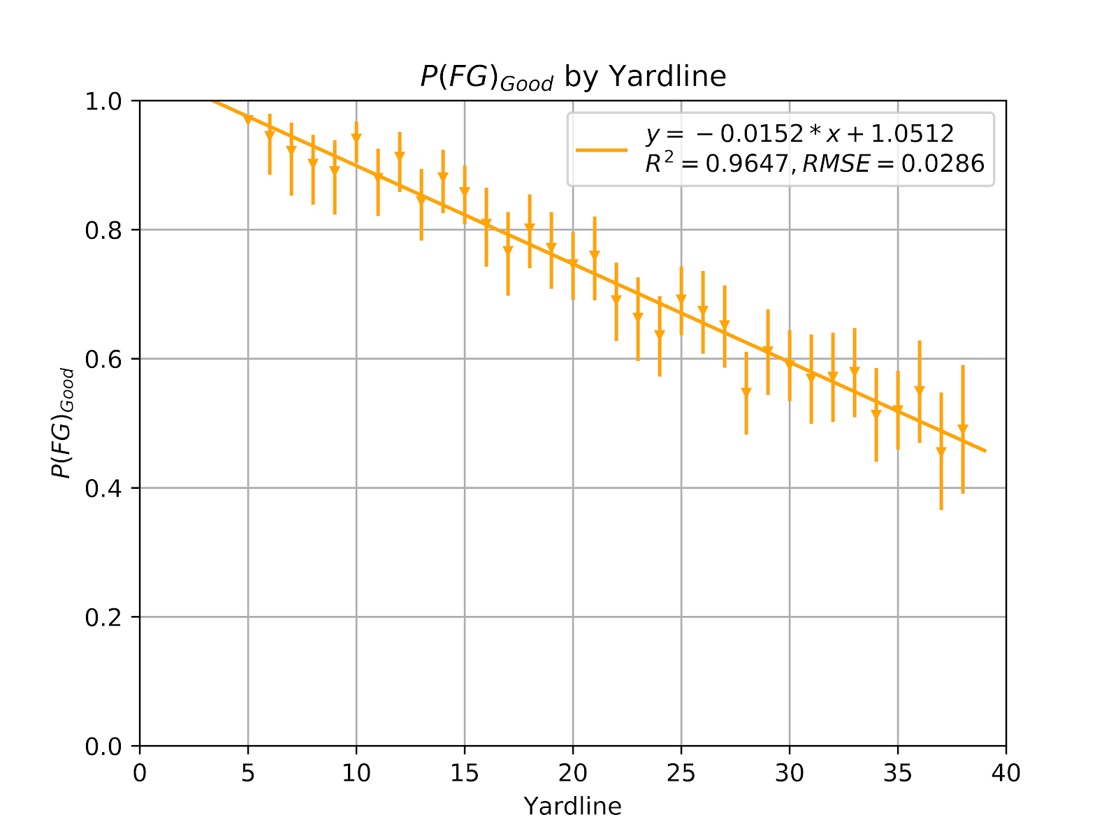
Figure 1 P(FG)Good by Yardline
Obviously the linear model proposed in Figure 1 is of no extrapolative value. The predicted probability is greater than 1 for yardlines less than 3, and gives negative probabilities beyond 70 yards. In principle the model would become asymptotic to 1 and small yardlines and asymptotic to 0, or debatably truly 0, at some large yardline. However, field goals are so rarely attempted outside the current dataset, and it serves no purpose to create models that are valid outside of their true domain. Simple linearity proves a very effective model here, passing through the 95% confidence window of each point save one. The threshold for minimum N here remains 100. Field goals within the five-yard line can be considered to have the same probability as attempts from the five. The convention used here is to consider the field position of the line of scrimmage of the kicking play, as this is the data that is consistently coded in the play-by-play. The actual kick itself is reliably seven yards greater than this.
A more comprehensive look at the outcomes of field goals is given in Figure 2, which shows good, missed, and rouge field goal rates by yardline. Note P(FG)ROUGE, which begins as a very low probability because few kicks are missed, then increases since most missed field goals will still reach the end zone, and then decreases as the number of field goals missed short increases, as does the number of missed field goals that are returned out of the end zone. This contrasts with the P(FG)GOOD, which is mostly monotonically decreasing, and P(FG)MISSED, which is mostly monotonically increasing with respect to yardline.

Figure 2 P(FG) by Yardline
b. EP
The calculation of the EP value of a field goal attempt is the mean value of the resultant EP of the play. Since the EP of a successful field goal is known (Clement 2019a), as is the EP value of a rouge, the calculation for these plays is trivial. For missed field goals the calculation is more complex. We must look at the EP value of the next play and consider which team has possession. This is simple enough to do in principle, but the actual code requires capturing a lot of edge cases with return touchdowns, return safeties, return turnovers (and some of these leading to offensive touchdowns) and other unique cases.
Some field goal attempts have penalties that lead to an offensive first down (e.g. roughing the kicker or offsides), so the EP contribution of that particular field goal is the value of the ensuing offensive play. Some models (Clement 2018c) opt to neglect the effects of missed field goals, which for American football reduces it to a binomial problem, but these penalties do occur, returns happen, blocks happen, and to neglect them is, in the author’s opinion, a bridge too far and a little too close to the proverbial spherical chicken (Stellman 1973).

Figure 3 EP(FG) by Yardline
Just as with the linear model in Figure 1, Figure 3 has a linear regression that breaks down, but only when pressed outside the expected domain. The error bars here are calculated by bootstrapping, necessary to incorporate missed field goals, and while they seem to be much tighter than in Figure 3, it should be noted that the range of the graph is five times the size, owing to the different units in play. Subjectively the two graphs are similar, unsurprising given that field goals can almost be reduced to a binomial distribution. The expectation of a field goal attempt is the most important result of this investigation, insofar as it will allow an apples-to-apples comparison of a coach’s options.
4. FG Models
Although Figure 3 gives the EP values of field goal attempts on average, field goal outcome probabilities are sensitive to certain contextual variables. In particular, this provides the first opportunity to factor in weather effects, using the highly granular data previously acquired (Clement 2019a, [a] 2018). Kicks were only included when all features were accounted for, as the sklearn models are not well-equipped to handle missing data. Additionally, all features are treated as continuous, since, again, sklearn does not fully support categorical data. Some of the models handle this inherently for continuous categorical data, such as the random forest and gradient boosting models, but models based on linear regression such as the logit model will treat these features as being purely continuous. This is less problematic in FG models than it was in EP models, as down is not a feature being considered here. Other libraries do exist which better handle categorical data, such as the H2O library (“H2O.ai Documentation” n.d.), but there are disadvantages to these libraries that make them unsuitable for a preliminary examination.
a. Features
i. Distance
Kick distance is consistently the most important variable, by far, in predicting FG success (Clement 2018c). This should come as no shock to anyone with even a passing familiarity with the game that field goals become more difficult as they become longer.
ii. Elevation
The elevation above sea level of the field is an attribute of the stadium object for a given game, as previously discussed (Clement 2019b). This is measured in metres. Increasing altitude leads to reduced air pressure and reduced air resistance on kicks. Elevation should show a small positive correlation with field goal success, especially at higher elevations, but this effect will be slight, and perhaps only field goals kicked in Calgary will show an impact. To get an even more accurate picture barometric readings could be used to even further adjust for air pressure but this would be a very slight adjustment of little consequence.
Because Calgary is the only stadium at significant altitude the data here will also be confounded by having most of the field goal attempts being taken by kickers from the University of Calgary. While this could be limited by only considering field goals of visiting kickers this would make the overall N of the model too small to consider altitude at all.
iii. Temperature
Cold weather is traditionally viewed as being more difficult for kicking, as all athletic activities become more difficult in the extreme cold. Beyond extremely cold temperatures, however, it is uncertain whether increasing temperature will have any impact on field goals. Previous assessments have used a boolean for very cold temperatures, but for a first assessment this has been left as raw temperature in degrees Celsius.
iv. Wind
While wind can be thought of as a simple constant vector, wind can be variable in both direction and speed. When the direction is variable this is noted in two ways: First, when wind speeds are low and directional variability is high, wind direction is noted not by a direction but by “VRB,” meaning “variable.” Here we consider both the headwind and crosswind components to be equal to the absolute value of the wind speed. When wind speeds are high and directional variability is low, the wind direction is noted by two bearings between which the wind is found. In this case the headwind and crosswind components are considered to be the maximum value within the range, calculated independently. These are in accordance with aviation rules regarding wind speeds and vectors (ICAO 3AD), as they may be taken to be the foremost authority on practical considerations of weather effects on flying objects. Where winds are gusty the wind speed is taken as the midpoint between the steady and gusty wind speed, following the same methodology (ICAO 3AD).
1. Headwind
Headwind is the vector component of the wind that runs parallel to the length of the field. Because the play-by-play lacks information about the direction that each offense is headed this is the absolute value of the headwind, and so we cannot tell if the wind is blowing for or against the kicker. We can assume that a wind blowing against the kick is always detrimental, and would be more so with increasing wind speed, but a wind blowing from behind the kicker would benefit the kick to a point, but we might also imagine that a very strong tailwind might induce more randomness than the benefit it provides. Being that most kicks occur in mild to moderate winds in either direction this feature is expected to be of little value.
2. Crosswind
Crosswind is the vector component of the wind that runs perpendicular to the length of the field. Because the play-by-play lacks information about the direction that each offense is headed this is the absolute value of the crosswind, and so we cannot tell if the crosswind is left-to-right or right-to-left, but this is much less of a concern than not knowing the direction of the headwind. In principle crosswind in either direction will have the same effect, and we should see P(FG)GOOD decreasing with respect to crosswind.
v. Weather
The notion of “weather” is meant to encompass all forms of weather that are not capture by wind and temperature, and so will encapsulate all manner of precipitation - rain, snow, sleet, hail - as well as such concepts as fog, smoke, or haze. More refined parsing could further differentiate all of these concepts, but would vastly increase the dimensional space of the model and would be difficult to quantify. While a blizzard and light mist are certainly not going to have the same effect on a kicker, it is as close as the current methodology can get with the data available.
There are a number of other features that could be considered in these models, such as the current score differential, home field advantage. However, there was a desire to keep this model agnostic of less-than-objective factors. The matter of “clutch kicking” has been debated endlessly (Clement 2018c), with the balance of the evidence implying that it has little effect, and certainly that it is harder to even define what is a clutch kick than to consider whether it matters. To keep the models tidy and avoid “kitchen sink-ing” the models these are omitted until such time as the number of models in consideration has been winnowed significantly and the question of “what is clutch” can be better assessed.
b. Models
The same models are used here as were used in the comparison of EP models, via largely the same methods and with thee same hyperparameters. These are taken from the sklearn library, the most popular library for such models (Pedregosa et al. 2011). This was done to create consistency and allow comparison of model efficacy in different contexts. The creation of the correlation graphs differs somewhat, however. For the EP correlation graphs the various multinomial outcomes were converted to an EP value given the value of each outcome multiplied by its probability. Here the probability of each outcome is plotted relative to the frequency of outcome. Thus, for each field goal three data points are created, the predicted outcomes of each of the three possible outcomes, and the true outcome is noted. A properly correlated model would show the same correlation graph as seen elsewhere, fitting y=x over the domain (0, 1).
This approach is chosen for two reasons over the approach used in the prior work. First, field goals are more concerned with which exact outcome, as the outcome is immediate and the impact of that outcome is often far more final than EP, where the idea is to optimize over a longer period. The second reason is that the value of a missed field goal is exceptionally difficult to value. The first goal of the model is and must be to predict the probability that a field goal attempt will be successful. Ergo the feature selection must be made with that as the main goal, hence the inclusion of wind and weather effects, along with altitude. These features, while useful for predicting field goal success probability, render the data overly granular to look at the result of missed field goals. Missed field goals also have a large degree of randomness, especially blocked kicks. Blocked kicks are not well-tracked in the source data. While some are noted, others are not, and the proportion is impossible to determine. We can accurately calculate the EP value of a field goal attempt and properly include the impact of blocks within it, with the bootstrapped confidence intervals considering the variance inherent in such plays. Thus, the models of field goals themselves need really only consider the probabilities of each of the three main outcomes - made, missed, or rouge.
Model
|
RMSE
|
R2
|
Logistic Regression
|
5.089
|
0.9658
|
k-Nearest Neighbours
|
4.941
|
0.9743
|
Random Forest
|
3.535
|
0.9858
|
Multi-Layer Perceptron
|
5.018
|
0.9648
|
Gradient Boosting Classifier
|
6.170
|
0.9460
|
Table 1 Correlation Metrics for FG Models
i. Logistic Regression (logit)
The one notable difference between this logit model and that used for EP (Clement 2019a) is that the max_iter argument was increased to 10,000, as 1,000 iterations was not enough to allow convergence. Logit has been a popular approach for modelling in the past, especially since it is well-suited to binomial response variables. Unfortunately Canadian football has the rouge, and it cannot be neglected if a model seeks to be more than a first approximation. Logit proved a poor fit for EP predictions (Clement 2019a) but that was largely due to compression effects.

Figure 4 Logistic Regression FG Correlation Graph
The logit model shows a good correlation in Figure 4, both visually and through the RMSE and R2 metrics. When reading a correlation graph in this context it is important to consider that the higher probabilities are dominated by predictions of successful field goals, and the lower predictions are for misses and rouges. In particular, recall from Figure 2 that P(FG)ROUGE runs from 0.0 to 0.2. Logit seems to overestimate the likelihood of misses, and underestimate the likelihood of success, over the majority of the model’s domain. Table 2 below shows the coefficients and intercepts of each feature.
Feature
|
GOOD
|
MISSED
|
ROUGE
|
Yardline
|
-0.0506
|
0.0385
|
0.0120
|
Elevation
|
0.0011
|
-0.0006
|
-0.0005
|
Temperature
|
0.0533
|
-0.0180
|
-0.0352
|
Headwind
|
0.0413
|
-0.0167
|
-0.0246
|
Crosswind
|
0.0586
|
-0.0170
|
-0.0415
|
Weather
|
0.1593
|
-0.0678
|
-0.0914
|
Intercept
|
0.8350
|
-0.4679
|
-0.3671
|
Table 2 Coefficients and Intercepts for Logistic Regression FG Model
Table 2 gives us a few obvious results, as we might expect. Every feature is correlated positively for GOOD, and negatively for both MISSED and ROUGE, which is unsurprising (yardline is vice-versa, negative for GOOD and positive for MISSED and ROUGE). This makes sense since we can see simplify field goals to a binary, with GOOD as one category and ROUGE as a subset of MISSED.
However, a number of features are perplexing. Crosswind has a positive correlation with FG success, the coefficient for headwind, which was expected to be near-zero given that only the absolute value is available, is 80% that of crosswind. Weather has a positive impact on FG success as well.
Some of these can be explained as a matter of selection bias. Strong headwinds against the kicker likely results in fewer overall attempts, while those in favour of the kicker may result in more overall attempts. Crosswind and weather can be explained by coaches overcompensating in the face of challenging conditions, and that above a certain threshold of crosswind very few FG attempts are likely to be seen. The impact of weather is difficult to quantify because the degree of weather is difficult to quantify, but an overcompensation theory seems the most likely.
ii. k-Nearest Neighbours (kNN)
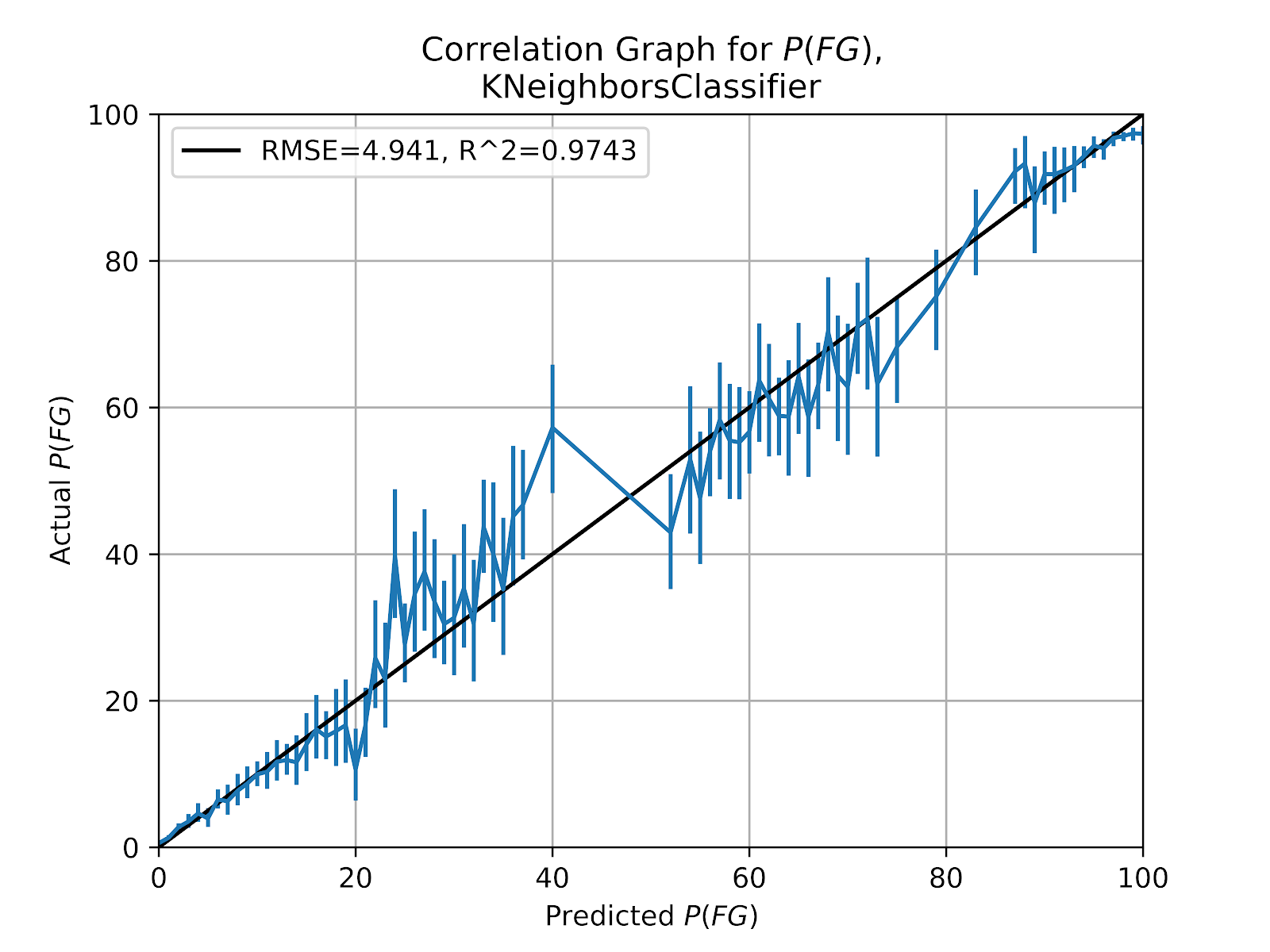
Figure 5 k-Nearest Neighbours FG Correlation Graph
At a glance, the kNN model in Figure 5 appears erroneous. There is a large gap between 40 and 50% with no data points. Consider first that the points on the correlation graph are only shown where N>100. As seen in Figure 2 there are few cases where raw P(FG)GOOD is less than 60%, or where P(FG)MISS is greater than 40%. There are few data points in that range, and so a number of the points in the correlation graph would not meet the minimum threshold. This is less a bug than a feature, showing that the model will not attempt to correlate to something it does not predict.
As with the EP model (Clement 2019a), this kNN model is entirely non-normalized, as a first order approximation. All of the factors are considered equal. Therefore some seemingly minor factors will have a disproportionate impact on the results. Yardline is known to be the most influential variable by far (Clement 2018c), and yet it’s range only extends from 0-50. Elevation varies over several hundred metres, but its impact is only truly felt at very high elevation (Clement 2018c). Weather has a not-insignificant impact on field goals, but as a boolean is only given the weight of a single yard, a single degree of temperature, or a single metre of elevation. In this model, 50 metres of elevation (an insignificant change) is weighted as much as 50m/s of crosswind - a literal tornado (Environment Canada 2013). By all rights, a kNN model should not work here, just as such a model should not have worked for EP. And while the kNN model for P(FG) is not nearly as good as for EP, it still proves remarkably capable as the second-best model by RMSE and R2. It is perhaps an indictment on data science’s fetishization of intricate models that a model whose method can be summarized as “averaging the ones that kind of look similar” can be as effective as more inscrutable methods.
A future effort would be to tune this model. A proper tuning effort would be rather laborious given the number of features to grid-search, but it could conceivably prove as effective as any more complex non-linear model.
iii. Random Forest (RF)
A random forest model would appear to be an ideal choice for this problem: A multiclass probabilistic classification problem with several features that are both non-linear and not independent. And indeed, Figure 6 confirms that RF is the best model for predicting P(FG) across the entire range. The model has the best correlation metrics, showing no evidence of bias or tendency.
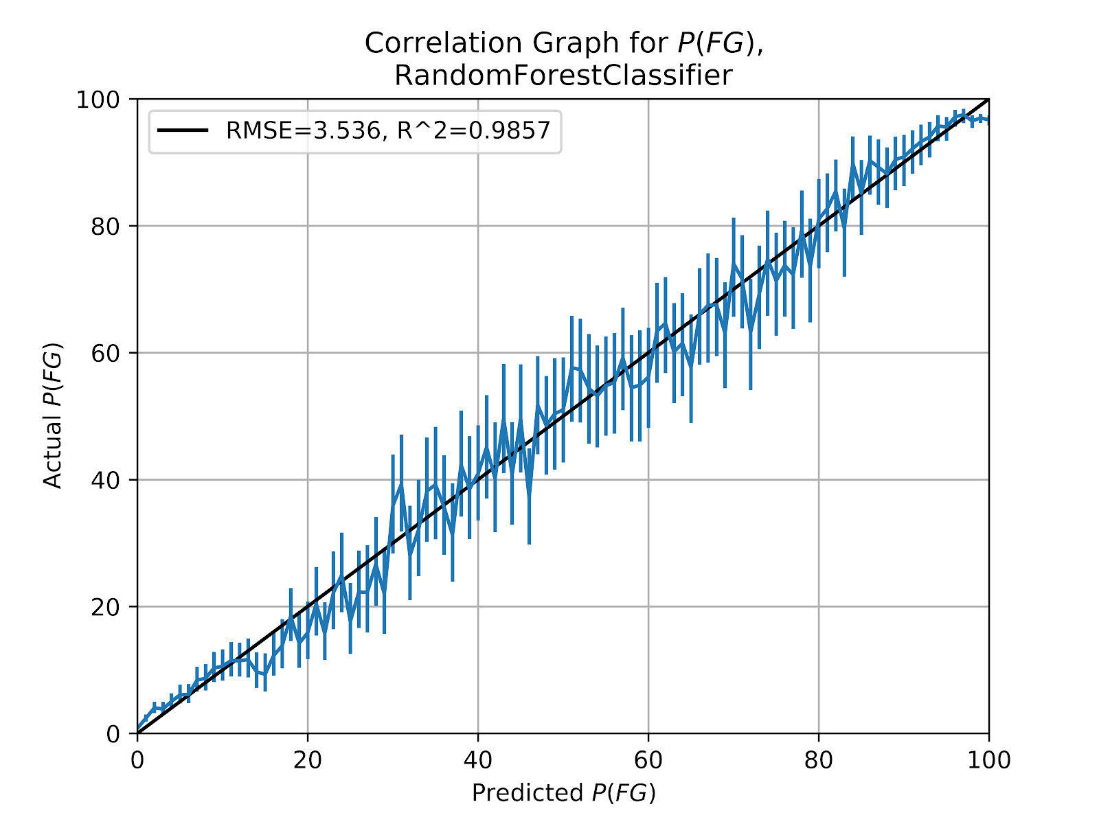
Figure 6 Random Forest FG Correlation Graph
A look at the feature importances in Table 3 gives more expected results than were seen for previous models. Unsurprisingly kick distance is the dominant feature. Wind, both headwind and crosswind, are the next-best feature. It remains unusual that headwind is such an effective predictor, as the lack of directional data means that headwind is only given as an absolute value. Crosswind would seem to be a more meaningful value, but the model’s results disagree.
Feature
|
Importance
|
Yardline
|
0.3291
|
Altitude
|
0.1181
|
Temperature
|
0.1520
|
Headwind
|
0.1903
|
Crosswind
|
0.1901
|
Weather
|
0.0201
|
Table 3 Feature Importance for RF FG Model
This sort of scenario is ripe for random forest - a large number of features blending continuous and categorical data on different scales that are all non-normally distributed. Thus it is no surprise that this model has strong metrics. We see kick distance as being a vastly stronger feature than its competitors, to no surprise. Again we see little distinction between the relevance of headwind and crosswind, and these are the two next most important features. It may simply be that wind strength itself is the factor that affects P(FG). Ideally this could be tested by having directional data available and testing the efficacy of models that consider the direction vs those that only consider the absolute values.
iv. Multi-Layer Perceptron (MLP)
MLPs are back-propagating neural networks that use linear relationships to determine class probabilities. This MLP has a very large node network relative to the domain space, larger than strictly necessary at (100, 100, 100). This model proved very useful for EP classification (Clement 2019a). The correlation graph for the MLP model is given in Figure 7.
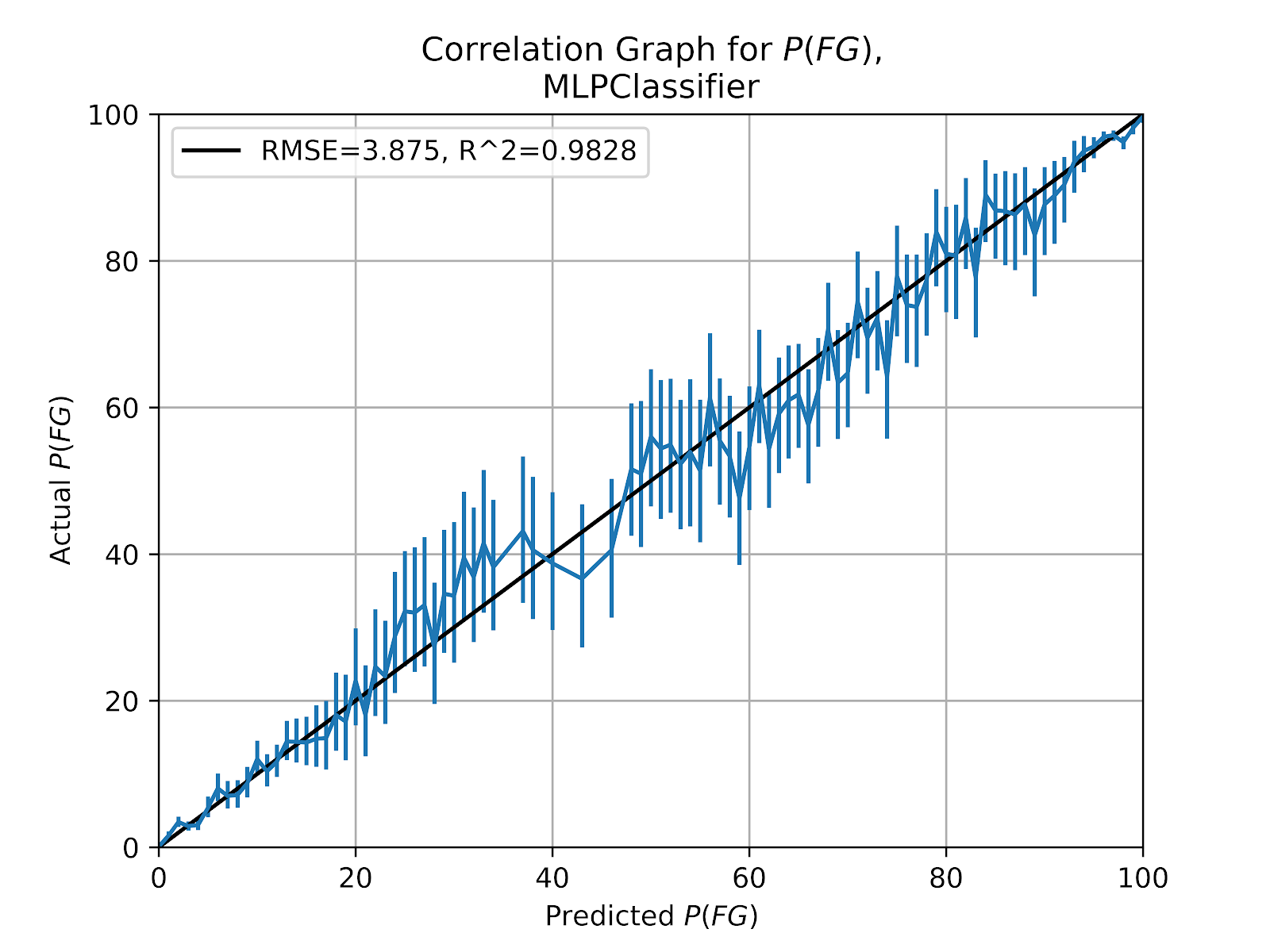
Figure 7 Multi-Layer Perceptron FG Correlation Graph
Figure 7 shows that the MLP shares something key in common with the kNN model - that they both consider the absence of probabilities in the 40-50% range in the raw data. All evidence both here and in prior work (Clement 2018c) point to kick distance as being the overwhelming predictive factor of P(FG). Looking at the outcome probabilities based purely on distance in Figure 2 there is a region between 40 and 50 yards that is underpopulated. If we consider the other features to be simply adjustments and modulations of the base probabilities brought on by kick distance then it is normal to expect few probabilities to be predicted in that range, hence the missing data points where they do not meet the threshold (N > 100), and the large confidence intervals where they do, signifying that even though N > 100, N is still relatively small compared to P(FG) at the extremes. From this we can draw that most FG attempts are fairly foregone conclusions. Ultimately the performance of the MLP seems disappointing, given its success in predicting EP outcomes under similar circumstances and the model’s vaunted reputation for resolving hidden connections
v. Gradient Boosting Classifier (GBC)
Gradient boosting models are a form of boosted trees model, a complexified form of the RF model. Hence we expect a better result than the simple RF model that, thus far, has shown the best results. The correlation graph for the GBC is given in Figure 8.

Figure 8 Gradient Boosting FG Correlation Graph
Disappointingly, the GBC does not compare to the simple efficacy of the RF model. The model is underconfident in kicker’s chances of making kicks, and overstates the likelihood of a miss or rouge. The feature importances, given in Table 4, provide insight into how the model arrived at its inferences.
Feature
|
Importance
|
Yardline
|
0.6790
|
Altitude
|
0.0547
|
Temperature
|
0.0503
|
Headwind
|
0.1036
|
Crosswind
|
0.4064
|
Weather
|
0.0056
|
Table 4 Feature Importance for GBC FG Model
Since GBC and RF models are related in their approach we would expect to see similarities in the way that they value different features. Instead, we see GBC put huge emphasis on kick distance, followed by crosswind. All other features were considered much less important, and weather was a non-factor.
5. Conclusion
Looking at the raw data of P(FG) based on distance alone shows that P(FG)GOOD and EP(FG) are both roughly linearly correlated over the domain of distances with sufficient data. It should be noted that at longer distances there will be some self-selection basis.
When looking at the five different models of P(FG) we see all five models produce passable results, but that the random forest model shows itself to be the clearly superior model, and should be the preferred model for this purpose going forward until such time as another model shows itself to be superior. Unlike EP where different models can argue to have different valid strengths and weaknesses there is little to argue that EP
Further work should seek to evaluate the cost of a missed field goal for a more nuanced understanding of the EP value of a field goal attempt. At shorter distances this distinction will be negligible, as most missed field goals will become rouges. Instead of using a classification model, this will use regression methods. Equivalent regression models for all of the models used here exist within Python’s sklearn library, which will allow for a more direct comparison of the models and how well they handle the more nuanced interpretation of EP(FG) versus P(FG).
An additional area of future study is risk optimization. Most field goals are fairly certain affairs, but it is not yet known whether coaches should take on greater risk in attempting less likely field goals without a better understanding of the outcome probabilities of the other options at a coach’s disposal.
6. References
Clement, Christopher M. 2018a. “It’s the Data, Stupid: Development of a U Sports Football Database.” Passes and Patterns. June 30, 2018. https://passesandpatterns.blogspot.com/2018/06/its-data-stupid-development-of-u-sports.html.
———. 2018b. “The Roman Numerals of Computing: An Object-Oriented Database of U Sports Football.” Passes and Patterns. October 13, 2018. https://passesandpatterns.blogspot.com/2018/10/the-roman-numerals-of-computing-object.html.
———. 2018c. “Three Point Plays: The Analytics of Field Goals.” Passes and Patterns. December 17, 2018. https://passesandpatterns.blogspot.com/2018/12/three-point-plays-analytics-of-field.html.
———. 2019a. “It’s Spelt ‘Rouge:’ Expected Points in U Sports.” Passes and Patterns. February 21, 2019. https://passesandpatterns.blogspot.com/2019/02/its-spelt-rouge-expected-points-in-u_21.html.
———. 2019b. “Home Sweet Home: Football Stadia in Canada.” Passes and Patterns. March 6, 2019. https://passesandpatterns.blogspot.com/2019/03/home-sweet-home-football-stadia-in.html.
———. 2019c. “Rain or Shine: Incorporating Weather Data into the U Sports Database.” Passes and Patterns. April 3, 2019. https://passesandpatterns.blogspot.com/2019/04/rain-or-shine-incorporating-weather.html.
Environment Canada. 2013. “Enhanced Fujita Scale for Wind Damage.” Government of Canada. May 10, 2013. https://www.canada.ca/en/environment-climate-change/services/seasonal-weather-hazards/enhanced-fujita-scale-wind-damage.html.


No comments:
Post a Comment