Passes and Patterns: New Year, New Data: Additions to the Passes and Patterns Knowledge Base

1. Abstract

An update on the developments affecting the various articles previously published in this space, covering both the analyses of other work and original research. Datasets for original research have been updated with 2018 data for both the CFL and U Sports. Previously written state of the art pieces that have seen new work in the field include a postscript to the original work to fold in the new research. Finally, original research previously done has been updated with the new data brought in.

The critical developments covered here include an American P(1D) (Pelechrinis and Papalexakis 2016b) model that shows non-linearity for 3rd down in a manner similar to that previously found in Canadian football (Clement 2018e, [g] 2018), and the development of a WP model for Canadian football (Thiel 2019).

2. Introduction

As the field of football analytics grows there is a constant stream of publication, research in new areas, work that builds upon existing knowledge, and replication of previous work. The three principal functions of this site are the synthesis of existing research, the development of new work, and the accumulation of machine-readable data to facilitate such work. Each year makes for new work in the field, an additional season’s worth of data, causing existing models to require updating and perhaps evolution. While publications are often considered frozen in time due to the historical difficulties in making updates to physical books, online publishing allows us to treat this continuously, rather than discretely.

3. New Data

a. It's the Data, Stupid: Development of a U Sports Football Database

All regular season and playoff games from the 2018 U Sports season were added, as well as several pre-season games that were played under normal rules. Pre-season games played under modified rules were not counted. The full list of games is given in Appendix A. Since the U Sports website uses Presto data but does not include the down & distance column it is impossible to use that source for play-by-play data. As a result data was extracted from the individual conference. For regular season and conference playoff games the play-by-play data was easily available on conference sites, in Data Format 1 (PrestoSports n.d.) for three conferences (CWUAA n.d.; OUA n.d.; AUS n.d.), while the fourth conference (RSEQ n.d.) uses Data Format 3 (The Automated Scorebook n.d.). Extensive manual and automated cleaning is still necessary because of both the limitations of the data formats and scoring errors. A small number of games were only available in Data Format 2, of unknown provenance.

b. Going Pro: Developing a CFL Play-by-Play Database

In contrast to the difficulties of U Sports data, enjoining the 2018 data (CFL n.d.) has proven relatively simple. The same scraper script was used as for the existing database (Clement 2018f) with the same tools for cleanup. The games added are available in Appendix B.

4. State of the Art

a. Keep the Drive Alive: First Down Probability in American Football

In studying the rationality of decision-making, 4th down conversion probabilities are obviously a relevant consideration. Most previous works have used 3rd down conversion rates as a proxy or have used the data from limited sample sizes for 4th down attempts (Clement 2018a). The use of 3rd down proxy was criticized by Krasker (2010), though without any specific suggestions to remedy the problem. Pelechrinis and Papalexakis (2016a) showed a much broader range and included confidence bands. A variation of these results was used in a later work (Pelechrinis 2018) and is shown in Figure 1.

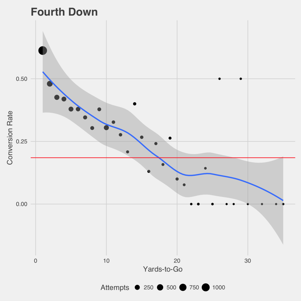
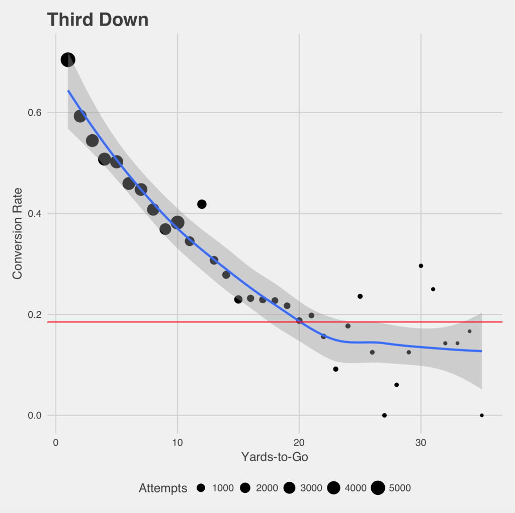
Figure 1 P(1D) for 4th Down (Pelechrinis 2018)

Pelechrinis (2018) would build on this in that same later work in discussing alternatives to the traditional kickoff, and compared the P(1D) of 4th down to that of 3rd down, shown in Figure 2. Unsurprisingly, the confidence bands are far narrower for 3rd down, with the much larger sample sizes. While other works have almost all shown 3rd down P(1D) as being linear with respect to distance (Clement 2018a), Figure 2 is decidedly non-linear, especially as distance grows past 20 yards. Instead we see similar results to what was shown in Canadian football, with both the CFL data (Clement 2018g) and especially the U Sports data (Clement 2018b). This was referred to as the “Stupidity Asymptote,” where P(1D) stops declining as defensive penalties become the dominant mode of conversion. This break from previous work in the field (Clement 2018a) through the use of more sophisticated statistical methods

Figure 2 P(1D) for 3rd Down (Pelechrinis 2018)

b. Score, Score Score Some More: Expected Points in American Football

Keith Goldner’s previously discussed Markov model of football EP (2011a) was in fact published in the Journal of Quantitative Analysis (Goldner 2012). Here Goldner goes into much greater detail in presenting his results, identifying the 340 bdata bins of down, distance, and field position and giving the absorption probabilities for each outcome. Goldner’s model remains a raw one, and so only considers scoring within a drive, and the use of the Markov method necessitates the use of binned data, but the method is an interesting take on the usual EP model.

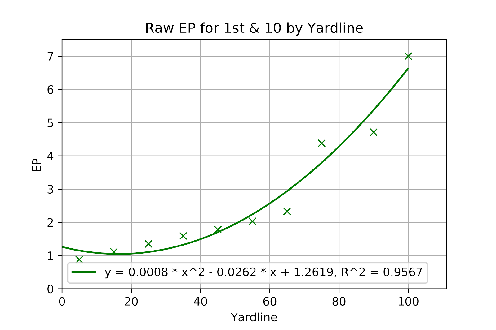
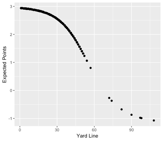
Another raw model was built to look at the expectations of different kickoff strategies (Urschel and Zhuang 2011). In it the author’s use a linear regression of their data, presumably under the (correct) assumption that EP models are generally linear between the 20 yard lines (Clement 2018b). Unfortunately, this assumption only holds for “complete” EP models that follow through until a scoring play or the end of a half. Raw models such as Goldner’s (2011b) that only consider scoring within a drive are generally quadratic in nature (Clement 2018c). Furthermore, complete EP models include negative values for the first 20 yards or so of field position, whereas raw models are never negative. We can only assume that the authors, while well-intentioned and perhaps viewing this model as a minor step toward their larger result, did not consider to plot their data. As shown in Figure 3, the data is visibly non-linear, and the quadratic curve is an excellent fit. Other similarly curved shapes, such as an exponential function, could also be considered here, but it is difficult to argue, given the lack of a physical justification, for a linear regression. The effect of this is to grossly overvalue field position in the middle of the field and undervalue it near the edges. Without fully recalculating the work of the original researchers it is impossible to determine exactly the impact of this change on the results.

Figure 3 Raw EP for 1st & 10 by Yardline (Clement 2019)

The use of raw EP as the measurement of choice for the value of field position in this context is itself dubious. Most drives do not end in points, but they do exchange field position, and that is neglected by raw models. A drive from the -10 that gains 40 yards before a punt is still a net positive for the offense, and will, over the long term, lead to positive results. This should and must be considered, particularly since the focus of the work was on non-necessary onside kicks, which are necessarily not performed near the end of games.

While looking to isolate the contributions of individual players, Yurko et al. (2018) developed an EP model based on a multinomial logistic regression with down and yardline as predictors, to the curious exclusion of distance. This is a complete response model of EP, including all future scoring, broken down by the probability of each scoring event. There is also a comparison of his model against some of the classic models of the past (Carter and Machol 1971; Carroll et al. 1998), with consistent results.

c. You Play to Win the Game: Win Probability in American Football

Along with the aforementioned EP model, Yurko’s (2018) team also developed a WP model. The concept is built around a Generalized Additive Model (GAM), which combines a series of linear models based on the various predictor variables. The GAM is best known for its interpolative power, a useful attribute since all future football plays exist within the state-space of past data, with limited exceptions for such things as extreme cases of distance to gain. Figure 4 gives the correlation graphs by quarter, showing the approximate accuracy of the model at different win probabilities. Correlation graphs are the most valuable tool in assessing such models at a glance, as they show regions where the model is failing either by over- or under-predicting the true WP.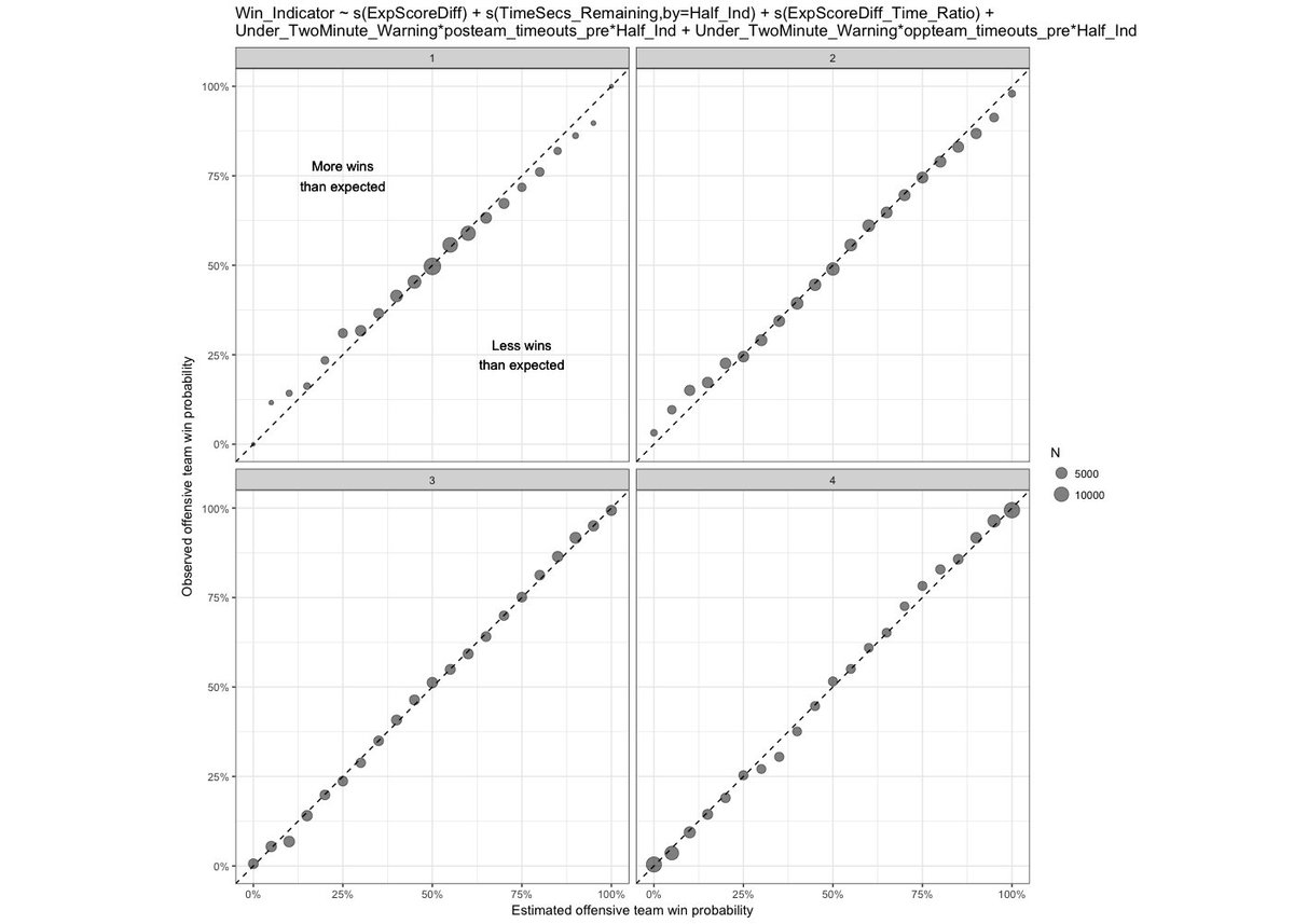

Figure 4 WP Correlation Graphs by Quarter (Ron Yurko 2017)

Given the popularity of this model is part of the larger nflWAR project (Ronald Yurko, Ventura, and Horowitz 2018) we may see more GAM models developed in the coming years, or perhaps an interest in other modelling techniques beyond the random forests and linear regressions seen in the past (Clement 2018d).

d. Due North: Analytics Research in Canadian Football

Although the work focuses on data from American football, the distinctly Canadian tone of the researchers’ previous work causes it to be included in this section (Brimberg and Hurley 2006). The conclusions of the work are indeed powerful, they find, with extraordinary statistical confidence, that football games are won and lost on the strength of the running game.They go so far as to recommend that teams design their teams around the running game and neglecting the pass game as “choosing a pass-dominated offense is, at best, a strategy that begs failure” (Brimberg and Hurley 2006). Indeed at first blush it is to difficult to refute their conclusions. The standard errors showing the positive correlation between running and winning, and the converse correlation for passing are vanishingly small, and we even see that rushing and turnovers are inversely correlated. The authors go so far as to suggest that a team should focus so heavily on the running game that they should not focus on turnovers, as turnovers are the product of poor rushing.

Unfortunately, the authors have fallen into a causality trap, indeed two. First, they have reversed the causality of their primary conclusion. Rushing yard do not lead to winning so much as winning leads to rushing yards. Running plays are a low-variance strategy that keep the clock running. Ergo, a team that is leading will call a disproportionate number of rushing plays as the game nears its conclusions. Conversely, teams that are trailing will attempt almost exclusively passes. Ergo, teams that are already winning will accumulate rushing yards as a product of their lead, and teams who trail will gain passing yards. The seeming effectiveness of rushing attacks is in fact an artefact of reversed causality.

By similar logic, the conclusion regarding turnovers is erroneous. Turnovers, more so than any other statistic, are correlated with winning. Teams who give away possession tend to lose games, and teams who take the ball away tend to lead. Ergo, we return to the same situation as above, where a team who leads adopts a rushing attack.

The first known Win Probability model for Canadian football was developed by Eric Thiel this year (2019). Similar to Yurko’s (2018) model, Thiel uses a GAM to determine win probabilities based on the current game state. Within the WP model is an EP model, not unlike others discussed in prior work (Clement 2018c). With 1st & 10 data shown in Figure 5, we see again the same more-or-less linear relationship between field position and expected points

Figure 5 1st & 10 Expected Points vs. Field Position (Thiel 2019)

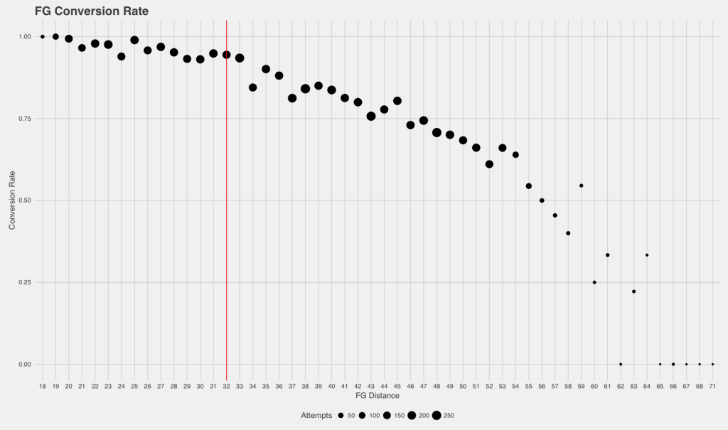
This author apologizes for the figure’s inversion of the usual axes for such EP graphs, but the point still remains: EP is largely linear with respect to field position. The use of EP in the model serves as a proxy for the game situation to simplify the WP model. The model considers score differential and EP rather than bringing in the distinct elements of down, distance, and field position. In this way it is similar to Paine & Lynch’s model (2013), which was known to suffer from issues regarding late-game discontinuities, where EP’s “perpetual first quarter assumption” breaks down (Clement 2018d). Evidence of the model’s performance is currently being prepared by the author and will have to be discussed at a later date. Within the model, scoring plays are taken at their nominal value, 7, 3, 2, or 1 point. Despite this, Thiel discusses the value of a kickoff as being worth 0.639, and goes into the development of a logistic regression model of field goal probability, represented as Expected Points but knowingly not accounting for the knock-on effects of missed field goals, shown in Figure 6. While logistic regression has often been used to model field goal success rates (Clement 2018i), it is used to incorporate different environmental factors into a single model. When modelling only distance logistic regression provides a poor fit to the data (Burke 2008)

Figure 6 EP(FG) by Field Position (Thiel 2019)

e. Kick it Away, Kick it Away, Kick it Away Now: The Analytics of Punting

Conducting yet another examination of the EP value of punts, Frye (2018) shows in Figure 7 the EPA value of punts by yardline. Unlike other works that showed the average resultant EP value of punts (Burke 2014), Frye uses the average EPA, the change in EP from the situation before and after the punt. While this is somewhat confounded by distance-to-gain as a hidden variable, it shows a different perspective. By considering the value of a position before a kick it considers the opportunity cost of the punt. Ergo, this chart has more in common with the 4th down decision charts than with the usual punt EP graphs, we see that punting has only modestly positive EP values throughout the zone where punting is the most commonly recommended approach, and goes negative as we reach the areas of the field where punting is contraindicated. We observe a slight oddity of punting EPA being negative when very backed up, within five yards of one’s end zone.

Figure 7 - Punting EPA by Yardline (Frye 2018)

f. Three Point Plays: The Analytics of Field Goals

Within their discussion of NFL decision-making, Pelechrinis & Papelaxis referred to (2016b) their visualization of field goal percentage by kick distance, which is the field position plus 17 yards - 10 yards because the goal posts are set at the back of the end zone, annd 7 yards because the kick is set back from the line of scrimmage.

Figure 8 P(FG) by Distance (Pelechrinis 2018)

Continuing the long-standing debate on icing the kicker, itself related to ongoing debates regarding clutch hitting in baseball and the hot hand effect in basketball, a new look supported the notion that icing the kicker has a meaningful effect, at least at longer distances (Dalen 2018). Positively, the analysis does make some effort to separate kicks by distance, but does not distinguish between which team called the timeout, nor whether the game situation constituted a proper icing situation. Additionally, given the large differences in sample sizes between the iced and non-iced kicks, the simple comparison of means is not an means of determining the statistical significance of the findings.

5. Original Research

a. Three Downs Away: P(1D) In U Sports Football

With the addition of the play-by-play data from the 2018 season the previous results for P(1D) in U Sports football could be updated (Clement 2018e). Although the quality of data entry in U Sports football has improved over the years, significant cleaning was still required. While small scripts and error-spotting tools simplified this task somewhat, a large portion of the effort was still manual. With the addition to the database the same code could be executed for updated results.

With the move from a relational database to an object-oriented one (Clement 2018h), regression functions were no longer determined through wizards or spreadsheet solvers, but instead through Python’s library scikit-learn (Pedregosa et al. 2011), using the scipy.optimize.curve_fit (Oliphant 2007) feature, aided by various numpy (Oliphant 2006) arrays. The results of this method are no different to results from the previous method.

Instead of simply plotting the data points meeting the N=100 threshold, attempts were made to use more sophisticated methods that could both incorporate all the data points and could be used to estimate P(1D) more accurately, even for points not included otherwise. The most popular choice for predicting a binary response variable is logistic regression, but logistic regression results proved to be far inferior to the previous methods, alternately grossly over- and under-estimating the experimentally verifiable results. After several attempts to use more sophisticated techniques the simpler approach of fitting a simple function with a least-squares regression to a plot of the data points best represented in the sample remains the most effective approach to showing the trends in P(1D) and to make small interpolations and extrapolations of the data.

The addition of a season of data pushed 2nd & 24 over the 100 data point mark, as had been predicted (Clement 2018e), and as is shown in Table 1. Therefore P(1D) is now complete for 2nd down for all distances up to 25 yards. No other data points were pushed over N=100. In fact, the point at 3rd & 11 has been removed due to improved filtering techniques that spot non-OD plays that otherwise would have tricked the parser, such as fake punts. Looking at Table 1, the only data point poised to be added in the near future is the reintroduction of 3rd & 11. Beyond that we might hope that some longer distances of 3rd down join the fold, and there may be a couple more data points beyond 25 yards on 2nd down worth considering.

Distance	1st Down	2nd Down	3rd Down
1	16	4688	3154
2	14	4184	843
3	9	4587	535
4	15	5204	443
5	963	6415	380
6	6	6120	282
7	8	6191	257
8	9	5738	193
9	12	4581	159
10	110713	20283	706
11	19	2850	98
12	30	2082	130
13	18	1485	72
14	34	1087	70
15	1844	1673	63
16	31	795	46
17	27	680	43
18	32	549	29
19	40	436	21
20	2592	1120	54
21	18	267	15
22	9	205	14
23	9	166	8
24	9	110	6
25	269	297	7

Table 1 Distribution of Data by Down and Distance for U Sports

Overall, and to no great shock, the P(1D) graph seen in Figure 9 appears unchanged. At a glance the two are virtually indistinguishable. With the data presented in tabular form in Table 2 there are modest increases for most down & distance pairings, a sign of a stronger year offensively than in the past.

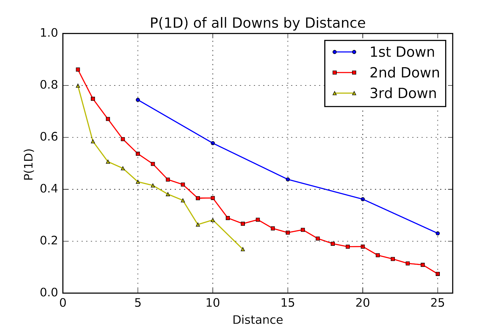
Figure 9 P(1D) of All Downs by Distance for U Sports

Distance	1st Down	2nd Down	3rd Down
1		0.8611	0.7993
2		0.7488	0.5848
3		0.6708	0.5065
4		0.5932	0.4808
5	0.7445	0.5370	0.4289
6		0.4977	0.4149
7		0.4376	0.3813
8		0.4183	0.3575
9		0.3658	0.2642
10	0.5776	0.3663	0.2819
11		0.2895
12		0.2675	0.1692
13		0.2828
14		0.2493
15	0.4381	0.2331
16		0.2440
17		0.2103
18		0.1905
19		0.1789
20	0.3618	0.1795
21		0.1461
22		0.1317
23		0.1144
24		0.1091
25	0.2304	0.0741

Table 2 DP(1D) for All Downs by Down and Distance for U Sports

i. 1st Down

A look at 1st Down shows that the linear correlation still exists. All data points have seen their P(1D) values increase, and of course the confidence intervals have shrunk slight due to the larger sample sizes. The across-the-board increase in P(1D) on 1st down raises the question of historiographical P(1D), and whether there has been a consistent, measurable increase over time. A look at the regression function shows that the slope is identical, but the intercept has increased slightly. A theoretically perfect model would have a y-intercept of 0, as at zero distance to gain a first down is already gained definitionally. But a theoretically perfect model also could never be a linear fit, as that raises the spectre of negative P(1D). Over the range of data that exists in practical applications this linear regression is the obvious choice, and allows for good interpolation and some limited extrapolation.

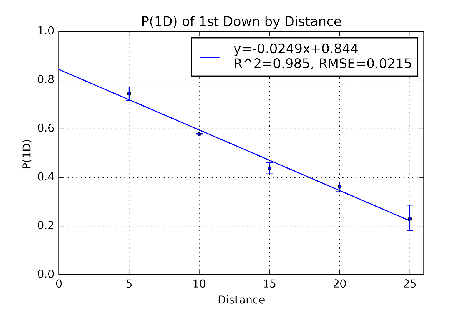
Figure 10 P(1D) for 1st Down by Distance for U Sports

Distance	Lower CL	P(1D)	Upper CL
5	0.7157	0.7445	0.7718
10	0.5747	0.5776	0.5805
15	0.4154	0.4382	0.4612
20	0.3433	0.3618	0.3806
25	0.1814	0.2304	0.2854

Table 3 P(1D) for 1st Down with 95% Confidence Intervals for U Sports

ii. 2nd Down

Of all P(1D) situations, 2nd down has shown the most visible change from the previous results. The addition of 2nd & 24 to the graph shows the complete set of data from 1 to 25 yards to gain. Figure 11 gives the graph of P(1D) for 2nd down, with 95% confidence intervals and the fitted curve. Table 4 gives a textual representation of the same data. Continuing with the exponential decay fit, we see the same general patterns as in the past; notably that 2nd & 10 outperforms expectations. The “stupidity asymptote” discussed at length in the past remains, but 25% lower than before. Hopefully future seasons will allow the inclusion of even longer distances to see if the trend holds. Future work could also look at the evolution of the asymptote over time to determine if we are seeing defensive evolution in response to this.

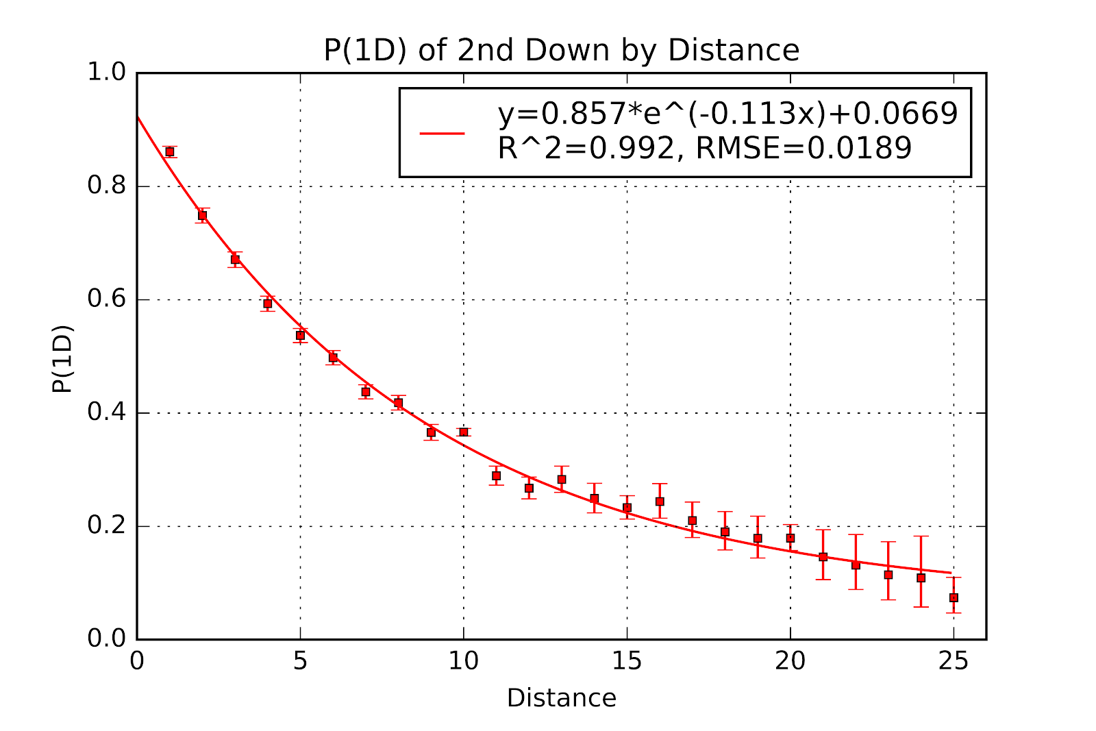
Figure 11 P(1D) for 2nd Down by Distance for U Sports

Distance	Lower CL	P(1D)	Upper CL
1	0.8509	0.8611	0.8709
2	0.7354	0.7488	0.7619
3	0.6570	0.6708	0.6844
4	0.5797	0.5932	0.6066
5	0.5246	0.5370	0.5492
6	0.4851	0.4977	0.5103
7	0.4252	0.4376	0.4500
8	0.4054	0.4183	0.4312
9	0.3519	0.3658	0.3800
10	0.3597	0.3663	0.3730
11	0.2729	0.2895	0.3065
12	0.2486	0.2675	0.2871
13	0.2600	0.2828	0.3065
14	0.2284	0.2493	0.2761
15	0.2130	0.2331	0.2541
16	0.2145	0.2440	0.2754
17	0.1805	0.2103	0.2429
18	0.1584	0.1905	0.2260
19	0.1440	0.1789	0.2182
20	0.1574	0.1795	0.2032
21	0.1060	0.1461	0.1942
22	0.0886	0.1317	0.1851
23	0.0703	0.1144	0.1730
24	0.0576	0.1091	0.1828
25	0.0470	0.0741	0.1100

Table 4 P(1D) for 2nd Down with 95% Confidence Intervals for U Sports

iii. 3rd Down

When compared to the original results, the visualization of 3rd down P(1D) shown in Figure 12 is beginning to resemble both 2nd down and our expectations of 3rd based on 2nd down. The asymptote of the exponential function is still too high to be plausible, and the issue with 3rd & 1 remains problematic, where 3rd & 1 is so often much less than one yard. More concerning is that P(1D) of 3rd down is almost certainly underestimated here because 3rd down attempts are vastly overrepresented by teams who are losing, and therefore generally worse than average.

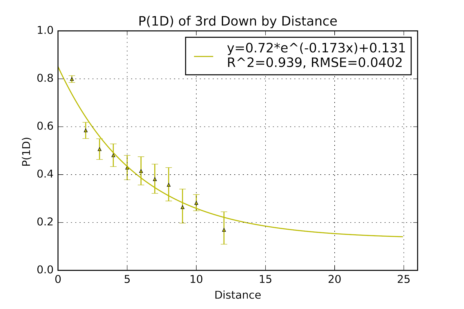
Figure 12 P(1D) for 3rd Down by Distance for U Sports

Distance	Lower CL	P(1D)	Upper CL
1	0.7849	0.7993	0.8132
2	0.5507	0.5848	0.6183
3	0.4633	0.5065	0.5497
4	0.4334	0.4808	0.5285
5	0.3786	0.4289	0.4804
6	0.3568	0.4149	0.4748
7	0.3217	0.3813	0.4437
8	0.2900	0.3575	0.4295
9	0.1975	0.2642	0.3398
10	0.2489	0.2819	0.3166
12	0.1092	0.1692	0.2449

Table 5 P(1D) for 3rd Down with 95% Confidence Intervals for U Sports

iv. & Goal

While no significant changes have occured for the & goal data, we remain curious about the sharp increase in P(1D) from 2nd & 5 to 2nd & 6. What may perhaps have been a statistical artefact has persisted for another year. This author remains surprised at the unwillingness of teams to attempt 3rd & Goal from the 2 yard line, and how 3rd & 1 remains the only point of 3rd & Goal to appear in Figure 13. 3rd & 2, even at 50% P(1D) would still be a far better proposition than kicking a field goal, worth an extra half-point. Given that 3rd & 2 for non-goal situations has a P(1D) of 58%, and that 3rd & 1 P(1D) is 78% for ordinary cases and 71% for & goal, seen in Table 6, a 50% P(1D) for 3rd & goal from the 2 is not an unreasonable proposition.

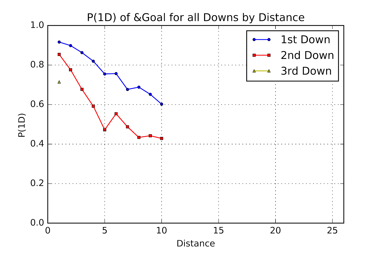
Figure 13 P(1D) of & Goal for All Downs by Distance for U Sports

Distance	1st Down	2nd Down	3rd Down
1	0.9163	0.8540	0.7143
2	0.8985	0.7763
3	0.8630	0.6770
4	0.8195	0.5918
5	0.7548	0.4723
6	0.7567	0.5536
7	0.6766	0.4876
8	0.6881	0.4337
9	0.6520	0.4423
10	0.6020	0.4286

Table 6 P(1D) of & Goal for All Downs by Distance for U Sports

b. The Whole Ten Yards: P(1D) in the CFL

As with U Sports, another CFL season passed in 2018, and with it a significant amount of new data to refine the P(1D) data. Two new points have been added to the graphs, having broached the N=100 threshold, at 2nd & 23 as well as 3rd & 12, shown in Table 7.

N	1st Down	2nd Down	3rd Down
1	12	3908	2449
2	2	3376	393
3	2	3736	247
4	3	4128	201
5	667	5054	187
6	2	4412	137
7	2	4249	92
8	5	3593	73
9	6	2840	69
10	82154	15621	410
11	7	1821	43
12	18	1340	102
13	28	904	72
14	19	695	60
15	1314	1266	55
16	12	486	29
17	12	447	27
18	19	412	19
19	13	318	16
20	1287	696	17
21	1	155	8
22		116	9
23	1	105	5
24	2	65	4
25	75	103	6

Table 7 Distribution of Data by Down and Distance for CFL

Unlike their U Sports counterparts, CFL offenses remained largely steady across all downs & distances for P(1D), with variations under 1% as the norm. The increased professionalization of the CFL vis-à-vis U Sports most likely contributes to this, and the improvement in average quarterback play seen in U Sports can be considered likely suspects.

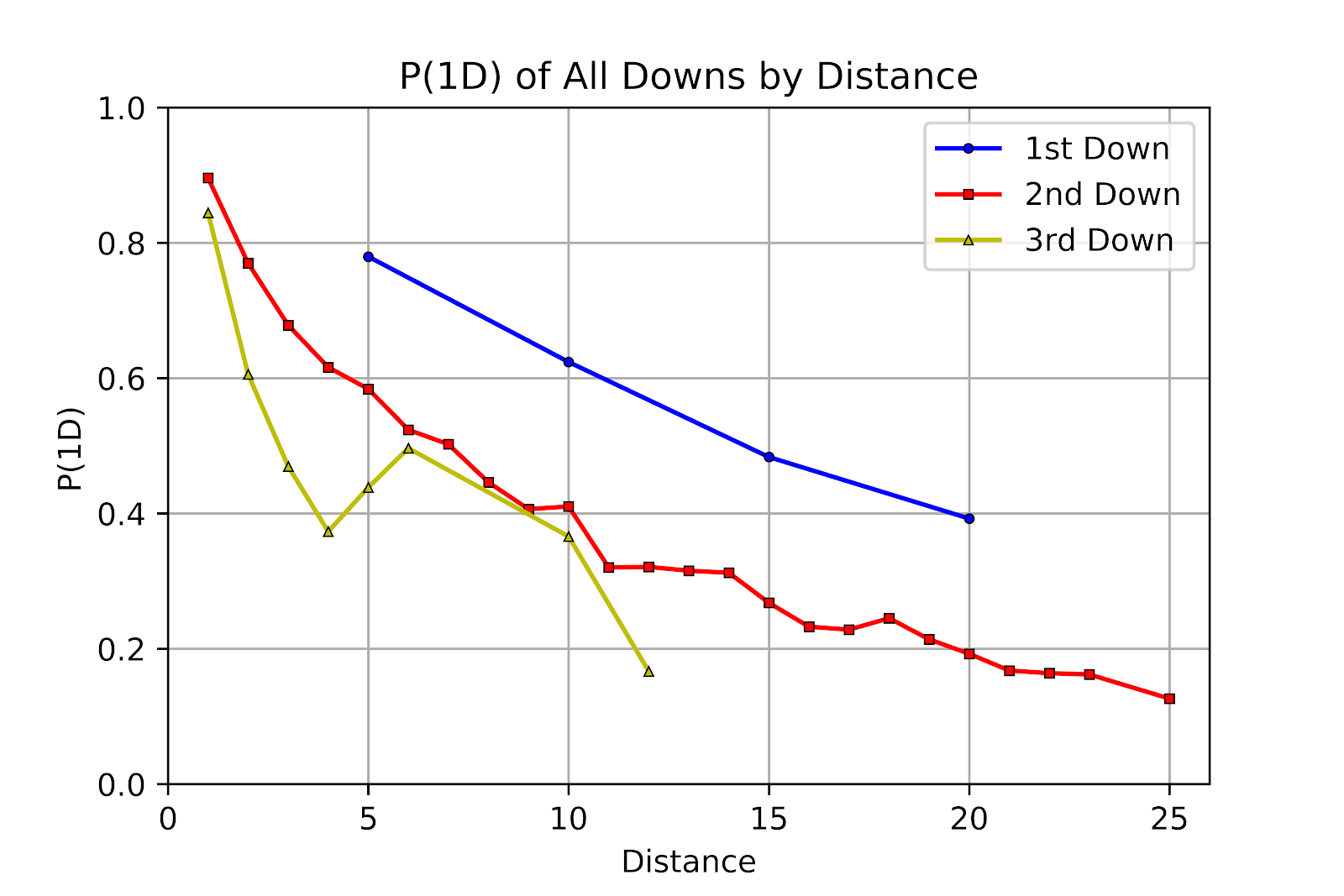
Figure 14 P(1D) for all Downs by Distance for CFL

Distance	1st Down	2nd Down	3rd Down
1		0.8959	0.8444
2		0.7698	0.6056
3		0.6783	0.4696
4		0.6160	0.3731
5	0.7796	0.5839	0.4385
6		0.5236	0.4964
7		0.5022	0.3261
8		0.4459	0.3288
9		0.4063	0.4783
10	0.6238	0.4103	0.3659
11		0.3202	0.2791
12		0.3209	0.1667
13		0.3153	0.2500
14		0.3122	0.2500
15	0.4833	0.2678	0.2182
16		0.2325	0.3103
17		0.2282	0.2593
18		0.2451	0.4211
19		0.2138	0.0625
20	0.3924	0.1925	0.1176
21		0.1677	0.0000
22		0.1638	0.2222
23		0.1619	0.4000
24
25	0.4133	0.1262	0.1667

Table 8 P(1D) for All Downs by Distance for CFL

i. 1st Down

In keeping with the theme of stability, the new graph of 1st down P(1D) in Figure 15 is almost indistinguishable from the previous one. In fact, the 95% confidence interval for 1st & 10 shown in Table 9 shrank by more than the average value moved.

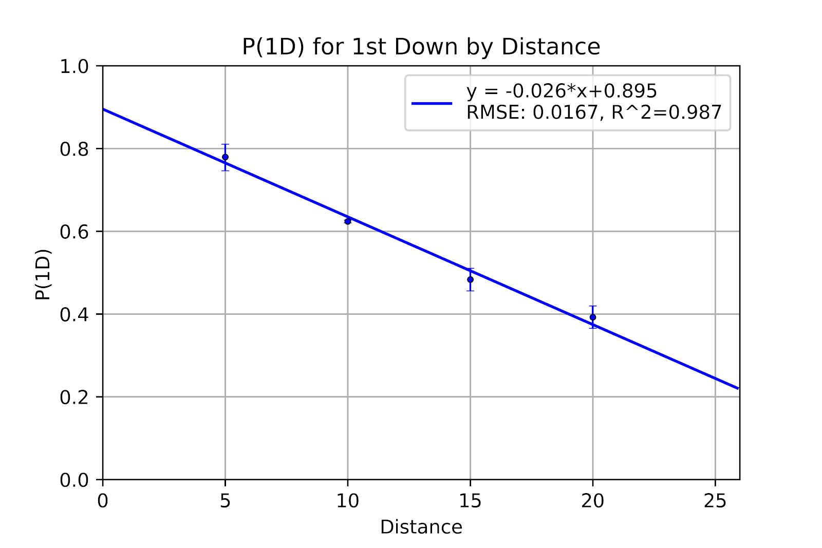
Figure 15 P(1D) for 1st Down by Distance for CFL

Distance	Lower CL	P(1D)	Upper CL
5	0.7462	0.7796	0.8105
10	0.6205	0.6238	0.6271
15	0.4559	0.4833	0.5107
20	0.3656	0.3924	0.4197

Table 9 P(1D) for 1st Down with 95% Confidence Intervals for CFL

ii. 2nd Down

2nd down shows a bit more movement than 1st down, with the addition of the point at 2nd & 23, seen in Figure 16. The asymptote has decreased slightly, and the R2 has improved. Certainly there have been no major changes in the general shape of the data. We do see a small generalized increase in P(1D), but this is too slight to make any commentary.

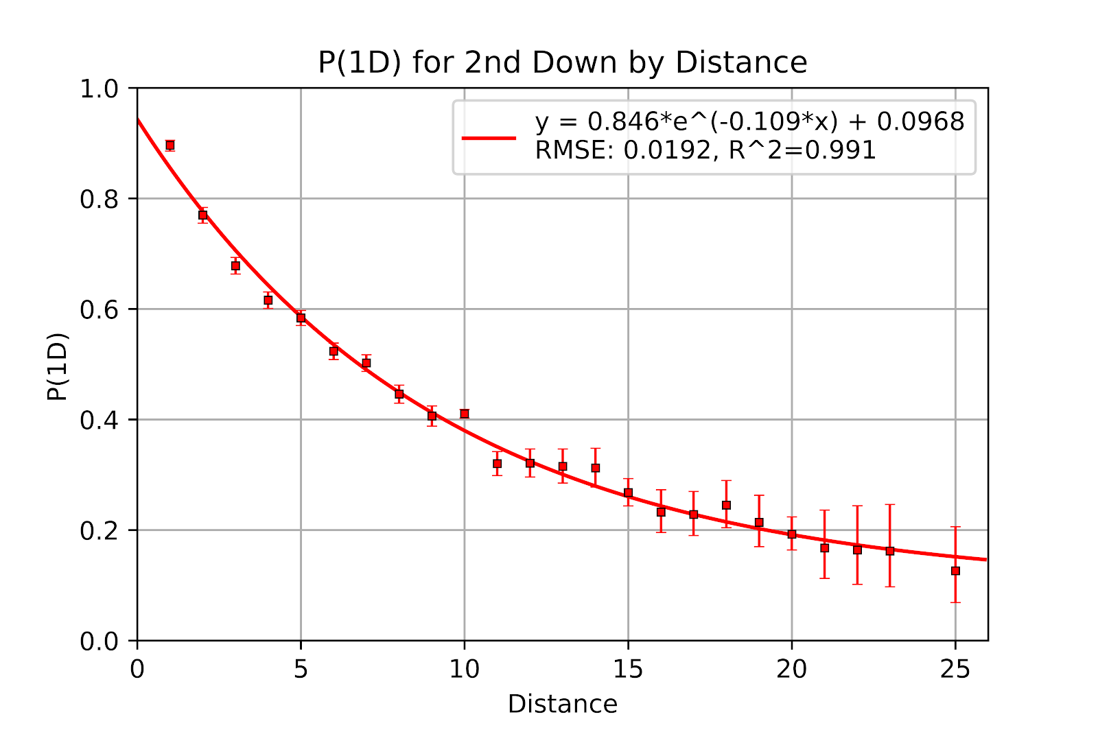
Figure 16 P(1D) for 2nd Down by Distance for CFL

Distance	Lower CL	P(1D)	Upper CL
1	0.8859	0.8959	0.9053
2	0.7553	0.7698	0.7840
3	0.6630	0.6783	0.6932
4	0.6010	0.6160	0.6309
5	0.5702	0.5839	0.5975
6	0.5087	0.5236	0.5384
7	0.4871	0.5022	0.5174
8	0.4295	0.4459	0.4623
9	0.3882	0.4063	0.4247
10	0.4026	0.4103	0.4180
11	0.2988	0.3202	0.3421
12	0.2959	0.3209	0.3466
13	0.2851	0.3153	0.3467
14	0.2779	0.3122	0.3481
15	0.2435	0.2678	0.2931
16	0.1956	0.2325	0.2727
17	0.1901	0.2282	0.2699
18	0.2044	0.2451	0.2896
19	0.1701	0.2138	0.2630
20	0.1639	0.1925	0.2238
21	0.1126	0.1677	0.2360
22	0.1016	0.1638	0.2439
23	0.0972	0.1619	0.2465
25	0.0689	0.1262	0.2062

Table 10 P(1D) for 2nd Down with 95% Confidence Intervals for CFL

iii. 3rd Down

Where the 3rd down graph previously defied any reasonable regression, the addition of 3rd & 12 in Figure 17 to our graph makes our regression seem to trend in the direction of common sense. CFL coaches remain incredibly hesitant to attempt 3rd down coaches. Without a significant cultural shift 3rd dow is likely to remain difficult to examine in any more detail. The confidence intervals remain very wide, generally too wide to make any broader statements. We cannot even begin to discuss the potential causes for 3rd & 6 being more prone to success than 3rd & 5.

Figure 17 P(1D) For 3rd Down by Distance for CFL

Distance	Lower CL	P(1D)	Upper CL
1	0.8295	0.8444	0.8586
2	0.5554	0.6056	0.6542
3	0.4061	0.4696	0.5339
4	0.3061	0.3731	0.4440
5	0.3662	0.4385	0.5128
6	0.4099	0.4964	0.5830
10	0.3191	0.3659	0.4145
12	0.1002	0.1667	0.2534

Table 11 P(1D) for 3rd Down with Confidence Intervals for CFL

iv. & Goal

When facing & goal situations P(1D) is lower than from other areas on the field. However, the general trends down-by-down seem to hold, at least for 1st and 2nd down. 3rd down, with its single point on Figure 18, cannot claim to have any sort of “trend.” 1st down remains roughly linear, while 2nd down follows a shape similar to the exponential decay of Figure 16. The most identifying feature on the 2nd down line is the sharp drop from 2nd & 1 to 2nd & 2, something which has been discussed at length (Clement 2018g). Oddly, 1st & 1 does not appear to exhibit the same stark dropoff. To the great dismay of both scientists nationwide, CFL coaches are steadfast in their unwillingness to attempt 3rd & goal, and so Figure 18 endures a privation of such data points.

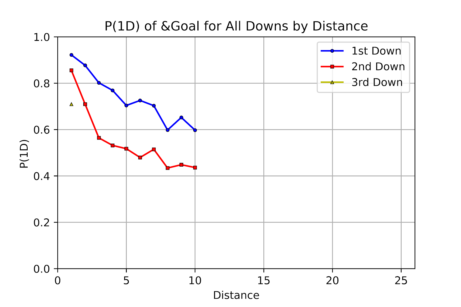
Figure 18 P(1D) of & Goal for All Downs by Distance for CFL

Distance	1st Down	2nd Down	3rd Down
1	0.9221	0.8555	0.7097
2	0.8770	0.7097
3	0.8018	0.5641
4	0.7690	0.5316
5	0.7039	0.5174
6	0.7256	0.4795
7	0.7031	0.5147
8	0.5979	0.4341
9	0.6522	0.4483
10	0.5974	0.4362

Table 12 P(1D) Data of &Goal for all Downs by Distance for CFL

6. Conclusion

Each year we hope for greater developments in football analytics, both improving existing concepts and pushing forward into new areas. With the growth in player GPS tracking it is becoming possible to examine plays at the player level, looking at three-space positioning of players and finding hidden patterns in the game. The most obvious applied uses are player evaluation metrics and in scouting, where teams can identify the unconscious tendencies of their opponents and seek to eliminate their own. The upcoming Big Data Bowl (NFL n.d.) will provide the first glimpse into the future of sports research.